$q_w=\frac{s}{4}$

$q_x=\frac{1}{s}(R_{32}-R_{23})$

$q_y=\frac{1}{s}(R_{13}-R_{31})$

$q_z=\frac{1}{s}(R_{21}-R_{12})$

else if $R_{11}>R_{22}$ and $R_{11}>R_{33}$ then

$s=2\sqrt{1+R_{11}-R_{22}-R_{33}}$

$q_w=\frac{1}{s}(R_{32}-R_{23})$

$q_x=\frac{s}{4}$

$q_y=\frac{1}{s}(R_{21}+R_{12})$

$q_z=\frac{1}{s}(R_{31}+R_{13})$

else if $R_{22}>R_{33}$ then

$s=2\sqrt{1+R_{22}-R_{11}-R_{33}}$

$q_w=\frac{1}{s}(R_{13}-R_{31})$

$q_x=\frac{1}{s}(R_{21}+R_{12})$

$q_y=\frac{s}{4}$

$q_z=\frac{1}{s}(R_{32}+R_{23})$

else

$s=2\sqrt{1+R_{33}-R_{11}-R_{22}}$

$q_w=\frac{1}{s}(R_{21}-R_{12})$

$q_x=\frac{1}{s}(R_{31}+R_{13})$

$q_y=\frac{1}{s}(R_{32}+R_{23})$

$q_z=\frac{s}{4}$

FIXME

$\delta=\text{trace}(\boldsymbol{R})$

if $\delta>0$ then

$s=2\sqrt{\delta+1}$

$q_w=\frac{s}{4}$

$q_x=\frac{1}{s}(R_{23}-R_{32})$

$q_y=\frac{1}{s}(R_{31}-R_{13})$

$q_z=\frac{1}{s}(R_{12}-R_{21})$

else if $R_{11}>R_{22}$ and $R_{11}>R_{33}$ then

$s=2\sqrt{1+R_{11}-R_{22}-R_{33}}$

$q_w=\frac{1}{s}(R_{23}-R_{32})$

$q_x=\frac{s}{4}$

$q_y=\frac{1}{s}(R_{21}+R_{12})$

$q_z=\frac{1}{s}(R_{31}+R_{13})$

else if $R_{22}>R_{33}$ then

$s=2\sqrt{1+R_{22}-R_{11}-R_{33}}$

$q_w=\frac{1}{s}(R_{31}-R_{13})$

$q_x=\frac{1}{s}(R_{21}+R_{12})$

$q_y=\frac{s}{4}$

$q_z=\frac{1}{s}(R_{32}+R_{23})$

else

$s=2\sqrt{1+R_{33}-R_{11}-R_{22}}$

$q_w=\frac{1}{s}(R_{12}-R_{21})$

$q_x=\frac{1}{s}(R_{31}+R_{13})$

$q_y=\frac{1}{s}(R_{32}+R_{23})$

$q_z=\frac{s}{4}$

### Action

$$\mathbf{R}_A^B~^A\mathbf{v}=^B\mathbf{v}$$

$$\mathbf{R}~^A\mathbf{v}=^A\mathbf{v}'$$

Composition and Inversion

Composition

$$\mathbf{R}_B^C\mathbf{R}_A^B=\mathbf{R}_A^C$$

Inversion

$$\left(\mathbf{R}_A^B\right)^{-1}=\left(\mathbf{R}_A^B\right)^T=\mathbf{R}_B^A$$

Addition and Subtraction

Perturbations are represented by $\boldsymbol{\theta}\in \mathbb{R}^3$, where local perturbations are expressed in the body frame and global perturbations are expressed in the world frame.

Addition

$$\boldsymbol{R}{B+}^{W}=\boldsymbol{R}{B}^{W} \text{Exp}\left(\boldsymbol{\theta}_{B+}^{B}\right)$$

$$\boldsymbol{R}{B}^{W+}=\text{Exp}\left(\boldsymbol{\theta}{W}^{W+}\right)\boldsymbol{R}_{B}^{W}$$

$$\boldsymbol{R}{W}^{B+}=\text{Exp}\left(\boldsymbol{\theta}{B}^{B+}\right)\boldsymbol{R}_{W}^{B}$$

Subtraction

FIXME

Notions of Distance

Angular/Geodesic

Gives the effective rotation angle about the correct axis:

$$||Log(\mathbf{R}_A^T\mathbf{R}_B)||=||Log(\mathbf{R}_B^T\mathbf{R}_A)||$$

Chordal

A computational, straight-line shortcut utilizing the Frobenius norm:

$$||\mathbf{R}_A-\mathbf{R}_B||_F=||\mathbf{R}_B-\mathbf{R}_A||_F$$

Derivatives and (Numeric) Integration

FIXME

Representational Strengths and Shortcomings

Strengths

• Excellent for calculations

Shortcomings

• Not very human-readable
• Clearly redundant with 9 numbers for a 3-DOF quantity

Unit Tests to Determine Conventions

FIXME

Euler Angles

Assuming 3-2-1 ordering.

Construction Techniques

From visualizing rotations from World to Body axes

First consideration: Order. Follow the exact order in a straightforward fashion.

Second, handedness must be considered:

Each rotation is visualized to be with respect to the transformed axes of the previous rotation.

Each rotation is visualized to be with respect to the world axes.

Handedness must be noted for all future operations with the numbers you just generated.

Conversions (To...)

This is the computational bedrock of the usefulness of Euler Angles. In fact, the Function and Directionality conventions only matter for conversions, and are dictated by the destination forms.

Rotation Matrix

See Rotation Matrix construction techniques for building the component $\mathbf{R}_i$ matrices here.

First consideration is directionality of the matrices (must be consistent):

$$\mathbf{R}_B^W=\mathbf{R}_3\mathbf{R}_2\mathbf{R}_1$$

$$\mathbf{R}_W^B=\mathbf{R}_1\mathbf{R}_2\mathbf{R}_3$$

$$\mathbf{R}=\mathbf{R}_3\mathbf{R}_2\mathbf{R}_1$$

Then, take into account handedness:

Keep the above, which was derived assuming successive axes.

Reverse the above, whatever it is:

$$\mathbf{R}_a\mathbf{R}_b\mathbf{R}_c \rightarrow \mathbf{R}_c\mathbf{R}_b\mathbf{R}_a$$

And the reversed rotations must be with respect to the chosen fixed frame. See below.

The aim is to prove that intrinsic and extrinsic rotation compositions are applied in reverse order from each other. To prove this, consider three frames 0,1,2, where 0 is the fixed "world" frame. Suppose that $\mathbf{R}_2^0$ represents the rotation of the 2-frame relative to the 0-frame. To encode that rotation relative to the 1-frame requires a similarity transform, granted that the frames no longer appear to cancel out nicely:

$$\mathbf{R}_2^1=(\mathbf{R}_1^0)^{-1}\mathbf{R}_2^0\mathbf{R}_1^0$$

Placing this within the context of rotation composition to get from frame 2 to 0, the composition looks like

$$\mathbf{R}_2^0=\mathbf{R}_1^0\mathbf{R}_2^1=\mathbf{R}_1^0((\mathbf{R}_1^0)^{-1}\mathbf{R}_2^0\mathbf{R}_1^0)=\mathbf{R}_2^0\mathbf{R}_1^0$$

Note the reversed directionality between the intrinsic composition $\mathbf{R}_1^0\mathbf{R}_2^1$ and the equivalent extrinsic composition $\mathbf{R}_2^0\mathbf{R}_1^0$. Generic rotations were used here, demonstrating generalizability.

Rodrigues

FIXME

Quaternion

FIXME

Composition and Inversion

Not applicable for Euler angles. Composition and inversion are typically performed by first converting the Euler angles to a rotation matrix.

Derivatives and (Numeric) Integration

Unlike with composition and inversion, there are methods of numeric differentiation and integration with Euler angles that are mathematically valid over infinitesimally small delta angles.

FIXME

Representational Strengths and Shortcomings

Strengths

• Can be very intuitive
• Minimal representation

Shortcomings

• There are many different orders and conventions that people don't always specify
• Operations with Euler angles involve trigonometric functions, and are thus slower to compute and more difficult to analyze
• //Singularities/Gimbal Lock//: For example, $\mathbf{R}=\mathbf{R}_z(\delta)\mathbf{R}_y(\pi/2)\mathbf{R}_x(\alpha+\delta)$ for any choice of $\delta$. Singularities will occur for any 3-parameter representation((J. Stuelpnagel. On the Parametrization of the Three-Dimensional Rotation Group. SIAM Review, 6(4):422-430, 1964.)).

Unit Tests to Determine Conventions

FIXME

Euler/Rodrigues

Construction Techniques

Remember, $\mathbf{u}$ is expressed in the World frame, just as you would intuitively think.

From Axis-Angle Representation: $\theta$, $\mathbf{u}$

Normalize $\mathbf{u}$ and multiply by $\theta$.

Conversions (To...)

//Besides tangent-space operations, this is the computational bedrock of the usefulness of Euler/Rodrigues.* In fact, as with Euler Angles, the Function and Directionality conventions only matter for conversions, and are dictated by the destination forms.

Rotation Matrix

i.e., the SO(3) exponential map.

*i.e., Rodrigues' rotation formula//.

$$\mathbf{R}B^W=\cos\theta\mathbf{I}+\sin\theta[\mathbf{u}]\times+(1-\cos\theta)\mathbf{u} \mathbf{u}^T$$

$$=\mathbf{I}+[\mathbf{u}]\times\sin\theta+[\mathbf{u}]\times^2(1-\cos\theta)$$

$$=exp([\theta\mathbf{u}]_\times)=Exp(\theta\mathbf{u})$$

$$\approx \boldsymbol{I}+\lfloor \boldsymbol{\theta} \rfloor_{\times}$$

FIXME

/(whatever the inverse of the other tab is ::::::::)*/

FIXME

Euler Angles

FIXME

Quaternion

i.e., the Quaternion exponential map.

Assuming O = $q_w$ first.

$$\mathbf{q}=\begin{bmatrix}\cos(\theta/2) \ \sin(\theta/2)\mathbf{u}\end{bmatrix}$$

FIXME

FIXME

Composition and Inversion

Composition

FIXME

Inversion

$$(\theta\mathbf{u})^{-1}=-\theta\mathbf{u}$$

Derivatives and (Numeric) Integration

FIXME

Representational Strengths and Shortcomings

Strengths

• Constitutes the Lie Group of SO(3).
• Easily visualized and understood
• Minimal representation

Shortcomings

• Similar to Euler Angles, operations are with trig functions, and thus slower to compute and harder to analyze (though the inverse is trivial to compute)
• Non-unique!

Unit Tests to Determine Conventions

FIXME

Quaternions

Construction Techniques

Because quaternions are so non-intuitive, it is generally best to construct a quaternion at the outset either as the identity rotation or converted from a different representation.

Conversions (To...)

Rotation Matrix

Hamiltonian cosine matrix:

$$\mathbf{R}=\mathbf{C}_H=(q_w^2-1)\boldsymbol{I}+2q_w\lfloor\boldsymbol{q}v\rfloor{\times}+2\boldsymbol{q}_v\boldsymbol{q}_v^{\top}=\begin{bmatrix}1-2q_y^2-2q_z^2 & 2q_xq_y-2q_wq_z & 2q_xq_z+2q_wq_y \ 2q_xq_y+2q_wq_z & 1-2q_x^2-2q_z^2 & 2q_yq_z-2q_wq_x \ 2q_xq_z-2q_wq_y & 2q_yq_z+2q_wq_x & 1-2q_x^2-2q_y^2\end{bmatrix}$$

/*::::see flipped quaternion paper::::

$$\mathbf{R}=\mathbf{C}_H=$$*/

FIXME

Shuster cosine matrix:

$$\mathbf{R}=\mathbf{C}_S=(q_w^2-1)\boldsymbol{I}-2q_w\lfloor\boldsymbol{q}v\rfloor{\times}+2\boldsymbol{q}_v\boldsymbol{q}_v^{\top}=\begin{bmatrix}1-2q_y^2-2q_z^2 & 2q_xq_y+2q_wq_z & 2q_xq_z-2q_wq_y \ 2q_xq_y-2q_wq_z & 1-2q_x^2-2q_z^2 & 2q_yq_z+2q_wq_x \ 2q_xq_z+2q_wq_y & 2q_yq_z-2q_wq_x & 1-2q_x^2-2q_y^2\end{bmatrix}$$

$$\mathbf{R}(\mathbf{q})=\mathbf{R}(-\mathbf{q}).$$

/* FIXME

(move to Lie tables?)*/

The use of $C_H$ means that $Exp(\tilde{q}) \approx I + [\tilde{q}]\times $ for small $\tilde{q}$. For $C_S$, the approximation becomes $I - [\tilde{q}]\times$. A transposed matrix flips the sign again. The sign change for the active + passive world-to-body convention is important because the values in the actual quaternion correspond to the inverse of the underlying passive quaternion. Thus, all Jacobians $\partial \cdot / \partial \tilde{q}$ must have that negated sign to send the linearizing derivatives in the correct direction given the apparent error-state value.

/:::Technically correct, but needs to be expanded from page 7 of notes.:::/

Euler Angles

FIXME

Rodrigues

FIXME

Action

Assuming O = $q_w$ last. Flip for $q_w$ first.

$$\mathbf{q}_A^B \otimes \begin{bmatrix}^A\mathbf{v}\0\end{bmatrix} \otimes \left(\mathbf{q}_A^B\right)^{-1}=^B\mathbf{v}$$

Homogeneous Coordinates:

$$\mathbf{q}_A^B \otimes \begin{bmatrix}^A\mathbf{v}\1\end{bmatrix} \otimes \left(\mathbf{q}_A^B\right)^{-1}=^B\mathbf{v}$$

FIXME

### Composition and Inversion

Composition

$$\mathbf{q}_1 \otimes \mathbf{q}_2=[\mathbf{q}_1]_L\mathbf{q}_2=[\mathbf{q}_2]_R\mathbf{q}_1$$

$$[\mathbf{q}]_L=\begin{bmatrix}q_w & -\mathbf{q}_v^T \ \mathbf{q}_v & q_w\mathbf{I}+[\mathbf{q}v]\times\end{bmatrix}=\begin{bmatrix}q_w & -q_x & -q_y & -q_z \ q_x & q_w & -q_z & q_y \ q_y & q_z & q_w & -q_x \ q_z & -q_y & q_x & q_w\end{bmatrix}$$

$$[\mathbf{q}]_R=\begin{bmatrix}q_w & -\mathbf{q}_v^T \ \mathbf{q}_v & q_w\mathbf{I}-[\mathbf{q}v]\times\end{bmatrix}=\begin{bmatrix}q_w & -q_x & -q_y & -q_z \ q_x & q_w & q_z & -q_y \ q_y & -q_z & q_w & q_x \ q_z & q_y & -q_x & q_w \end{bmatrix}$$

$$[\mathbf{q}]_L=\begin{bmatrix}q_w\mathbf{I}+[\mathbf{q}v]\times & \mathbf{q}_v\-\mathbf{q}_v^T & q_w\end{bmatrix}=\begin{bmatrix}q_w & -q_z & q_y & q_x\q_z & q_w & -q_x & q_y\-q_y & q_x & q_w & q_z \ -q_x & -q_y & -q_z & q_w\end{bmatrix}$$

$$[\mathbf{q}]_R=\begin{bmatrix}q_w\mathbf{I}-[\mathbf{q}v]\times & \mathbf{q}_v\-\mathbf{q}_v^T & q_w\end{bmatrix}=\begin{bmatrix}q_w & q_z & -q_y & q_x\-q_z & q_w & q_x & q_y\q_y & -q_x & q_w & q_z \ -q_x & -q_y & -q_z & q_w\end{bmatrix}$$

$$[\mathbf{q}]_L=\begin{bmatrix}q_w & -\mathbf{q}_v^T \ \mathbf{q}_v & q_w\mathbf{I}-[\mathbf{q}v]\times\end{bmatrix}=\begin{bmatrix}q_w & -q_x & -q_y & -q_z \ q_x & q_w & q_z & -q_y \ q_y & -q_z & q_w & q_x \ q_z & q_y & -q_x & q_w \end{bmatrix}$$

$$[\mathbf{q}]_R=\begin{bmatrix}q_w & -\mathbf{q}_v^T \ \mathbf{q}_v & q_w\mathbf{I}+[\mathbf{q}v]\times\end{bmatrix}=\begin{bmatrix}q_w & -q_x & -q_y & -q_z \ q_x & q_w & -q_z & q_y \ q_y & q_z & q_w & -q_x \ q_z & -q_y & q_x & q_w\end{bmatrix}$$

$$[\mathbf{q}]_L=\begin{bmatrix}q_w\mathbf{I}-[\mathbf{q}v]\times & \mathbf{q}_v\-\mathbf{q}_v^T & q_w\end{bmatrix}=\begin{bmatrix}q_w & q_z & -q_y & q_x\-q_z & q_w & q_x & q_y\q_y & -q_x & q_w & q_z \ -q_x & -q_y & -q_z & q_w\end{bmatrix}$$

$$[\mathbf{q}]_R=\begin{bmatrix}q_w\mathbf{I}+[\mathbf{q}v]\times & \mathbf{q}_v\-\mathbf{q}_v^T & q_w\end{bmatrix}=\begin{bmatrix}q_w & -q_z & q_y & q_x\q_z & q_w & -q_x & q_y\-q_y & q_x & q_w & q_z \ -q_x & -q_y & -q_z & q_w\end{bmatrix}$$

When attaching frames to the quaternions, composition has the potential for nuance due to the fact that, in certain implementations, a quaternion can be specified to represent a certain type of SO(3) rotation that actually uses different conventions from the quaternion. This seems unwise, but it happens, as with certain manifestations of the JPL convention. For that reason, one cannot simply exclusively pair Passive B2W behavior with active behavior, as other combinations are also fair game.

$$\mathbf{q}_A^C=\mathbf{q}_B^C\otimes \mathbf{q}_A^B$$

$$\mathbf{q}_A^C=\mathbf{q}_B^C\otimes \mathbf{q}_A^B$$

$$\mathbf{q}_A^C=\mathbf{q}_A^B\otimes \mathbf{q}_B^C$$

Inversion

$$\mathbf{q}^{-1}=\begin{bmatrix}q_w\\mathbf{q}_v\end{bmatrix}^{-1}=\begin{bmatrix}q_w\-\mathbf{q}_v\end{bmatrix}$$

$$\left(\mathbf{q}_a \otimes \mathbf{q}_b \otimes \dots \otimes \mathbf{q}_N\right)^{-1}=\mathbf{q}_N^{-1}\otimes \dots \otimes \mathbf{q}_b^{-1} \otimes \mathbf{q}_a^{-1}$$

Addition and Subtraction

/* (:::copy to Lie tables?:::)

::With addition and subtraction, an additional convention is introduced--that of global vs. local perturbations:: FIXME integrate right-and-left subtraction/addition operations for quaternions and others--should make a lot of sense when thinking about rotation matrices!. In other words, are the increments defined in the local (i.e., body frame) tangent space, or in the global (i.e., inertial/world frame) tangent space? FIXME The combination of passive directionality with this additional convention determines how $\oplus$ and $\ominus$ are expressed. When you write out the frames, it makes sense. Take $\mathcal{I}$ as the global frame/tangent space and $\mathcal{B}$ as the local. Here are some combinations, using rotation matrices:

• Passive B2W + Local Perturbations: $R_\mathcal{B_t}^\mathcal{I}=R_\mathcal{B}^\mathcal{I} Exp\left(\tilde{\theta}_\mathcal{B_t}^\mathcal{B}\right)$.
• Passive B2W + Global Perturbations: $R_\mathcal{B}^\mathcal{I_t}=Exp\left(\tilde{\theta}\mathcal{I}^\mathcal{I_t}\right)R\mathcal{B}^\mathcal{I}$.
• Passive W2B + Local Perturbations: $R_\mathcal{I}^\mathcal{B_t}=Exp\left(\tilde{\theta}\mathcal{B}^\mathcal{B_t}\right)R\mathcal{I}^\mathcal{B}$.

Note that (and this is very easy to miss) while the rotation matrix form of our convention follows the third bullet point, the quaternion in our convention is active, which means it behaves like a body-to-world rotation operator! So, when dealing in the space of quaternions, the first bullet point is actually used! Effectively, for our convention, quaternions compose in the opposite way that rotation matrices do. Very tricky. FIXME

:::add notion of error rotation...same for other representations!::: */

FIXME

Notions of Distance

Quaternion distance

$$||\mathbf{q}_A-\mathbf{q}_B||=||\mathbf{q}_B-\mathbf{q}_A||$$

A modification to account for the negative sign ambiguity:

$$\min_{b\in{-1;+1}}||\mathbf{q}_A-b\mathbf{q}_B||$$

Derivatives and (Numeric) Integration

FIXME

Representational Strengths and Shortcomings

Strengths

• Minimal representation with no singularities!
• Fast computation without resorting to trigonometry
• Composition has 16 products instead of 27 for rotation matrices

Shortcomings

• Not as intuitive as Euler Angles
• Sign ambiguity poses challenges that must be circumvented in control and estimation problems

Unit Tests to Determine Correctness

FIXME

/* FIXME for Hamiltonian convention, main tests for Transform3D def for Ceres notes

q1 = Quaterniond(0.,1.,0.,0.) q2 = Quaterniond(0.,0.,1.,0.)

print('q1:\n')
print(q1)
print('\nq2:\n')
print(q2)
print('\nq1.inv():\n')
print(q1.inverse())
print('\nq1*q2:\n')
print(q1*q2)
print('\nq2*q1:\n')
print(q2*q1)


T1 = Transform3D().Random()
T2 = Transform3D().Random()

print('\nT1:\n')
print(T1)
print('\nT2:\n')
print(T2)
print('\nT1-T2:\n')
print(T1 - T2)
print('\nT2-T1:\n')
print(T2 - T1)
print('\nT1+(T2-T1)=T2:\n')
v = T2-T1
print(T1 + v)
print('\nT2-(T1+(T2-T1))=0:\n')
print(T2 - (T1 + (T2-T1)))

*/ ## Appendix

More info on quaternions found here((Some UPenn notes on quaternions)).

Linear Algebra

• Visualizing Matrices

Visualizing Matrices

There are various scenarios (e.g., covariance matrices, inertia matrices, quadratic forms) in which you'd want to represent a (square) matrix visually, and ultimately it comes down to Eigen decompositions.

In graphics, it's generally preferable to draw an "unrotated" version of your graphic, and then apply a rotation. Thus, the methods below will focus on extracting semi-major axis lengths and a rotation from the Eigen decomposition. Example code will be given in Matlab.

For testing, here's some Matlab code for generating a random \(n\times n\) positive-definite matrix:

function A = generateSPDmatrix(n)
% Generate a dense n x n symmetric, positive definite matrix

A = rand(n,n); % generate a random n x n matrix

% construct a symmetric matrix using either
A = 0.5*(A+A'); OR
A = A*A';
% The first is significantly faster: O(n^2) compared to O(n^3)

% since A(i,j) < 1 by construction and a symmetric diagonally dominant matrix
%   is symmetric positive definite, which can be ensured by adding nI
A = A + n*eye(n);

end

Two/Three-Dimensional Positive Definite Matrix (Ellipse/Ellipsoid)

Matrix: \(\boldsymbol A\in \mathbb{R}^{2\times 2}\) or \(\boldsymbol A\in \mathbb{R}^{3\times 3}\), \(\boldsymbol A > 0\)

Get the principal axis lengths:

• Find eigenvalues of \(\boldsymbol A\). These are the (ordered) semi-major axis lengths.
  • Let's say that by convention, \(\boldsymbol A\) is expressed in frame \(W\), and when it's expressed in frame \(F\), it's diagonal (\(\boldsymbol D\)) with the eigenvalues on the diagonal.

Get the rotation matrix:

• Find the (ordered) eigenvectors of \(\boldsymbol A\). These form the column vectors of \(\boldsymbol R_F^W\).
• Check the determinant of \(\boldsymbol R_F^W\); if it's -1, then flip the sign of the last column to make the determinant +1.
• From matrix basis change rules, you can check your work by making sure that \(\boldsymbol D=\left(\boldsymbol R_F^W\right)^{-1}\boldsymbol A\boldsymbol R_F^W\).

Matlab code:

% Get random positive definite matrix
A = generateRandom2x2PDMatrix();

% Extract axis lengths and rotation
[R,D] = eig(A);
x_axis_len = D(1,1);
y_axis_len = D(2,2);
if det(R) < 0
    R(:,2) = -1 * R(:,2);
end

% Draw unrotated ellipse
theta = linspace(0,2*pi,100);
coords = [x_axis_len * cos(theta); y_axis_len * sin(theta)];
plot(coords(1,:),coords(2,:),'k--')
hold on; grid on

% Draw rotated ellipse (R acts like active rotation
% since it's B2W convention)
rotated_coords = R * coords;
plot(rotated_coords(1,:),rotated_coords(2,:),'k-','Linewidth',2.0)
hold off

A

function A = generateRandom2x2PDMatrix()
A = rand(2,2);
A = A*A';
A = A + 2*eye(2);
end

$$\boldsymbol A=\begin{bmatrix}3.0114 & 0.9353 \\ 0.9353 & 2.9723\end{bmatrix}$$

Systems Implementation

• Computer Simulations
  • The Rotor Blade Flapping Effect
  • Event-Based Collision Detection
  • The Intertial Measurement Unit (IMU) Sensor
• Optimization Libraries
  • Ceres Solver Python Tutorial (Linux)
  • 2D Range-Bearing Landmark Resolution with Ceres

Computer Simulations

• The Rotor Blade Flapping Effect
• Event-Based Collision Detection
• The Intertial Measurement Unit (IMU) Sensor

The Rotor Blade Flapping Effect

Source Papers

• [LIT] Quadrotor Helicopter Flight Dynamics and Control: Theory and Experiment
  • Considers four aerodynamic effects which arise when deviating significantly from hover flight regime
  • Taking them into account allows for improved tracking at higher speeds and in gusting winds
• [LIT] Propeller Thrust and Drag in Forward Flight
• [LIT] Aerodynamics and Control of Autonomous Quadrotor Helicopters in Aggressive Maneuvering
• [LIT] Improved State Estimation in Quadrotor MAVs: A Novel Drift-Free Velocity Estimator
  • focuses on the translational force that opposes quadrotor motion
  • actually uses it to get more accurate velocity estimation

Consolidated Model

Core Equations

A rotor in translational flight undergoes an effect known as blade flapping. The advancing blade of the rotor has a higher velocity relative to the free-stream, while the retreating blade sees a lower effective airspeed. This causes an imbalance in lift, inducing an up and down oscillation of the rotor blades. In steady state, this causes the effective rotor plane to tilt at some angle off of vertical, causing a deflection of the thrust vector (see Figure 2). If the rotor plane is not aligned with the vehicle’s center of gravity, this will create a moment about the center of gravity ($M_{b,lon}$) that can degrade attitude controller performance. For stiff rotors without hinges at the hub, there is also a moment generated directly at the rotor hub from the deflection of the blades ($M_{b,s}$).

The total moment on the UAV about the body pitch and roll axes comes from the contribution of each rotor $i$:

$$M_{flap,\phi}=\sum_i (M_{b,lon,\phi,i}+ M_{b,s,\phi,i})$$

$$M_{b,lon,\phi,i}=T_ih\sin{a_{1s,\phi}}$$

$$M_{b,s,\phi,i}=k_\beta a_{1s,\phi}$$

$$a_{1s,\phi}=-k_f~^bv_y$$

$$M_{flap,\theta}=\sum_i (M_{b,lon,\theta,i}+ M_{b,s,\theta,i})$$

$$M_{b,lon,\theta,i}=T_ih\sin{a_{1s,\theta}}$$

$$M_{b,s,\theta,i}=k_\beta a_{1s,\theta}$$

$$a_{1s,\theta}=k_f~^bv_x$$

Where

$h$ is the vertical distance from rotor plane to origin of the body frame ($m$),

$k_\beta$ ::is the stiffness of the rotor blade:: ($N~m/rad$),

$k_f$ ::is a constant providing a linear approximation to Eq. 8 on page 7 of [1]. The linear approximation is explained preceding Eq. 14 on page 4 of [3]::.

Additionally, the total force on the quadrotor is

$$^\mathcal{I}F_{flap}=-\lambda_1\sum_i\omega_i\tilde{V}$$

Where

$\omega_i$ is the rotational speed of each rotor,

$\tilde{V}$ is the projection of $^\mathcal{I}V$ on to the propeller plane,

$\lambda_1$ is a “critical parameter” which is the rotor drag coefficient, and ::probably entails an experimental estimation method (introduced on page 37 of [4])::

Manipulating the relations from the top left of page 35 of [4], there is an easier-to-estimate parameter (again, see page 37) called $k_1$ (::which is assumed to be constant throughout stable flight::) such that

$$ k_1=\lambda_1\sum_i\omega_i. $$

The authors of [4] found their $k_1$ value to be equal to 0.57.

Motor thrust related to total angular rotation rate by the following relation (::from page 33 of [4]::):

$$T=k_T\sum_i\omega_i^2$$

where $k_T$ is the "thrust coefficient" of the propellers.

How to simulate effect

Currently, we are using a Force-Torque polynomial model fit to go directly from PWM motor commands to output thrusts and torques. This gives us no information about the individual rotor speed without an estimate of $k_T$. If all the rotor planes were parallel with each other, this would not be a big deal if we had a reasonable estimate of $k_1$. However, since our rotor planes are not guaranteed to be parallel, we need to use the following process to compute the blade flapping effect forces and torques on the UAV:

This is roughly what I'm doing in C++:

<code c++> double omega_Total = 0.0; for (int i = 0; i < num_rotors_; i++) { ... motor_speeds_(i, 0) = sqrt(abs(actual_forces_(i) / motor_kT_)); omega_Total += motor_speeds_(i, 0); }

• Blade flapping effect for (int i = 0; i < num_rotors_; i++) {

  • determine allocation of k_1 to each motor and calculate force and torques double k1i = motor_k1_ * motor_speeds_(i, 0) / omega_Total;

  • Calculate forces Force_ -= k1i * (Matrix3d::Identity() - motors_[i].normal*motors_[i].normal.transpose()) * airspeed_UAV;

  • Calculate torque about roll axis double as1phi = -motor_kf_ * airspeed_UAV(1); Torque_(0) -= actual_forces_(i) * motors_[i].position(2) * sin(as1phi); Torque_(0) += motor_kB_ * as1phi;

  // Calcualte torque about pitch axis double as1theta = motor_kf_ * airspeed_UAV(0); Torque_(1) -= actual_forces_(i) * motors_[i].position(2) * sin(as1theta); Torque_(1) += motor_kB_ * as1theta; }

Parameter Estimation Attempts

Rotor Blade Stiffness $k_\beta$

Page 15 of this thesis gives a static bending test table for a nylon 6 rotor blade, Under a load of 0.9 N, the measured deflection at the tip of the blade (with a length of 6 in = 0.1524 m) was 0.0305 m. Numerous other load and deflection values were tabulated. The calculated elastic modulus from the table was 9.5 GPa.

Given the above numbers, $k_\beta$ can be calculated as

$$k_\beta=\frac{(0.9N)(0.1524m)}{\tan^{-1}(0.0305m/0.1524m)}\approx 0.7 \frac{Nm}{rad}.$$

/*To find an estimate for $k_\beta$, an examination of its units plus the information we're given has us ask the question: for a load of 1 N applied at a point 1 meter out on the rotor blade, what will the angular deflection be? (I will use scaling to make the numbers more realistic, with a load of 1 N at a point 0.1 meter out. We will use the cantilever beam deflection formula:

$$\delta = \frac{FL^3}{3EI}.$$

where the deflection angle $\theta$ is equal to $\tan^{-1}(\delta/L)$. A sample from the table will allow us to calculate an approximate value for the moment of inertia I, which is calculated to be 3.75 $mm^4$. We can thus calculate that if a load of 1 N will be applied 0.1 meter out from the rotor blade*/

Rotor Thrust Coefficient $k_T$

From this paper, it is noted that quadrotors tend to have very low thrust coefficients compared to helicopters (on the order of zero from looking at the figure on page 20). As a ballpark estimate, the paper explains that the quadrotors studied require motor speeds around 5000 RPM to keep the vehicle in the air. Assuming that a quadrotor's mass is somewhere around 2 kilograms and distributed evenly among four rotors, that would give a thrust coefficient of

$$k_T=\frac{F_{rotor}}{\omega^2}\approx 2.0 \times 10^{-5} \frac{N s^2}{rad^2}$$

which is in line with the figure.

The Enigmatic $k_1$ Parameter

I'm just copying the empirical value from [4] here, though it might be interesting in the future to replicate their parameter estimation process for our own platform if deemed necessary.

$$k_1 \approx 0.57 \frac{kg~rad}{s}$$

Event-Based Collision Detection

Predict and handle a collision before it happens rather than make adjustments after the fact.

Planar Case

Sources

• [1] [[https://algs4.cs.princeton.edu/61event/]]

[1] assumes all disks move in straight lines without any external forces or anything other than single-integrator dynamics. Then, you can form your global priority queue with impending collisions. This assumption can be circumvented by (assuming your simulation has a time step $\Delta t$) doing the same logic but limiting your sense of time to the time window $t=0\rightarrow \Delta t$ and resetting your priority queue at every time step. In fact, you can chop your normal simulation time step into a bunch of smaller $\Delta t$'s if the straight-line trajectory assumption holds up better over those smaller time steps.

^ Symbol ^ Meaning ^ | $p=\begin{bmatrix}p_x & p_y\end{bmatrix}^T$ | Agent position at start of time window. | | $v=\begin{bmatrix}v_x & v_y\end{bmatrix}^T$ | Agent velocity at start of time window. | | $r$ | Agent radius | | $\pm h$ | y-limits where wall is located. | | $\pm w$ | x-limits where wall is located. |

For each time window:

Initialize discard list $\mathcal{D}={(\text{time},\text{agent index})}$ to empty.

Form priority queue $\mathcal{P}={[\tau](\text{time-of-insertion},\text{agent(s)},\text{collision TYPE})}$, which sorts by time-to-collision $\tau$. Queue items can take the form of a special collision class.

For each agent $i$:

If $v_y$ > 0:

$\tau=(h-r-p_y)/v_y$

If $\tau \leq \Delta t$: Append [$\tau$](0,$i$, WALL-UP) to $\mathcal{P}$

Else If $v_y$ < 0:

$\tau=(-h+r-p_y)/v_y$

If $\tau \leq \Delta t$: Append [$\tau$](0,$i$, WALL-DOWN) to $\mathcal{P}$

If $v_x$ > 0:

$\tau=(w-r-p_x)/v_x$

If $\tau \leq \Delta t$: Append [$\tau$](0,$i$, WALL-RIGHT) to $\mathcal{P}$

Else If $v_x$ < 0:

$\tau=(-w+r-p_x)/v_x$

If $\tau \leq \Delta t$: Append [$\tau$](0,$i$, WALL-LEFT) to $\mathcal{P}$

For each pairwise combination (order doesn't matter) $(i,j)$ of agents:

$\Delta p = p_j-p_i$

$\Delta v = v_j-v_i$

$\sigma = r_i + r_j$

$d=(\Delta v \cdot \Delta p)^2-(\Delta v \cdot \Delta v)(\Delta p \cdot \Delta p - \sigma^2)$

If $\Delta v \cdot \Delta p < 0$ and $d \geq 0$:

$\tau = -\frac{\Delta v \cdot \Delta p + \sqrt{d}}{\Delta v \cdot \Delta v}$

If $\tau \leq \Delta t$: Append [$\tau$](0,$(i,j)$, INTER-AGENT) to $\mathcal{P}$

Work through priority queue:

While $\mathcal{P}$ not empty:

Grab collision from top of queue.

If time-of-insertion < an item in $\mathcal{D}$ with a matching agent ID, then simply discard and delete (also the item in $\mathcal{D}$).

Else: Simulate all agents in the simulation and advance global time up to $t=\text{time-of-insertion}+\tau$.

Remove all items in $\mathcal{D}$ with time < $t$.

Carry out collision type and remove from $\mathcal{P}$.

Append to $\mathcal{D}$ tuples of $t$ and the agents involved.

For each agent involved, repeat all of the $\mathcal{P}$ append logic, replacing the insertion time with $t$.

$$\boldsymbol{\beta}{k}=\boldsymbol{\beta}{k-1}+\mathcal{N}(0,\sigma_{\beta})\Delta t,$$

$$\boldsymbol{\eta}{\boldsymbol{k}}=\mathcal{N}(0,\sigma{\eta}),$$

where $\mathcal{U}$ and $\mathcal{N}$ are the uniform and normal distributions.

Shifting Measurements in $SE(3)$

Suppose we want an IMU measurement model for when the IMU is mounted away from the inertially-centered body frame, still rigidly attached to the vehicle. We have an $SE(3)$ transform description of the relationship between the body frame and this "shifted" frame, which we'll refer to as $U$: $$\boldsymbol{T}{U}^{B}=\begin{bmatrix}\boldsymbol{R}{U}^{B} & \boldsymbol{t}_{U/B}^{B}\ \boldsymbol{0} & 1 \end{bmatrix}.$$

We will now derive the shifted accelerometer measurement $\bar{\boldsymbol{a}}^{U}$ in terms of the body-frame measurement $\bar{\boldsymbol{a}}^{B}$. Applying Eq. (A.1), the shifted measurement would be $$\bar{\boldsymbol{a}}^{U}=\left(\boldsymbol{R}{U}^{W}\right)^{\top}\left(\frac{d\boldsymbol{v}{U/W}^{W}}{dt^{W}}-\boldsymbol{g}^{W}\right)+\boldsymbol{\eta}^{U}+\boldsymbol{\beta}^{U}. $$

Before proceeding, there are two key things to note from basic kinematics:

• Because both $B$ and $U$ are rigidly attached to the same vehicle, $$\boldsymbol{\omega}{U/W}=\boldsymbol{\omega}{B/W}.$$
• A frame with a non-zero offset away from the vehicle center of mass will experience additional velocity under vehicle rotation: $$\boldsymbol{v}{U/W}=\boldsymbol{v}{B/W}+\boldsymbol{\omega}{B/W}\times\boldsymbol{t}{U/B}.$$

Applying these two facts, the shifted measurement can be re-written as \begin{align*} \bar{\boldsymbol{a}}^{U} & =\left(\boldsymbol{R}{U}^{B}\right)^{\top}\left(\bar{\boldsymbol{a}}^{B}+\frac{d}{dt^{W}}\left(\boldsymbol{\omega}{B/W}^{B}\times\boldsymbol{t}{U/B}^{B}\right)\right)\ & =\left(\boldsymbol{R}{U}^{B}\right)^{\top}\left(\bar{\boldsymbol{a}}^{B}+\frac{d}{dt^{B}}\left(\boldsymbol{\omega}{B/W}^{B}\times\boldsymbol{t}{U/B}^{B}\right)+\boldsymbol{\omega}{B/W}^{B}\times\left(\boldsymbol{\omega}{B/W}^{B}\times\boldsymbol{t}_{U/B}^{B}\right)\right).\ \end{align*}

Expanding the derivative and triple product terms, the concise shifted accelerometer measurement equation is

The shifted rate gyro equation involves only a frame change:

Optimization Libraries

• Ceres Solver Python Tutorial (Linux)
• 2D Range-Bearing Landmark Resolution with Ceres

Ceres Solver Python Tutorial (Linux)

Ceres Introduction

The Ceres Solver () is Google's powerful and extensive C$++$ optimization library for solving:

• general unconstrained optimization problems
• nonlinear least-squares problems with bounds (not equality!) constraints.

The second application is particularly useful for perception, estimation, and control in robotics (perhaps less so for control, depending on how you implement dynamics constraints), where minimizing general nonlinear measurement or tracking residuals sequentially or in batch form is a common theme. This is further facilitated by Ceres' support for optimizing over vector spaces as well as Lie Groups, much like GTSAM. To zoom in on the comparison between the two libraries a bit, here are some relative pros and cons:

^ Ceres Advantages ^ GTSAM Advantages ^ |

• Supported by Google, not just one research lab
• Has an awesome automatic differentiation system--no time wasted computing complicated derivatives
• Generalizes well beyond robotics applications, or even exotic robotics applications that don't yet have pre-programmed tools |
• Made specifically for robotics applications, so comes with a lot of useful tools, such as:
• iSAM2 incremental optimization
• Marginalization support (e.g., for fixed-lag smoothing) |

Aside from what's mentioned in the table, GTSAM adopts the helpful [docs](http://deepdive.stanford.edu/inference|factor graph]] modeling paradigm for estimation problems. If desired, Ceres can be used through the definition of factors as well, as will be shown in the examples below. All in all, Ceres is a fine choice for solving optimization-based inference problems, and it's not going away any time soon. Moreover, the [[http://ceres-solver.org/) are thorough and well-made; this tutorial can be thought of as an entry point to give some context to a deep-dive into the documentation.

Solving Problems with Ceres

At a minimum, a Ceres program for solving nonlinear least-squares problems requires the following specifications:

• A Problem() object.
• For every decision variable ("parameter") that isn't a vector:
  • Add a LocalParameterization() object to the problem using the function AddParameterBlock().
• For every residual in the problem:
  • Add a CostFunction() object (can be thought of as a factor in factor graph lingo) with the relevant parameters using the function AddResidualBlock()

See the examples below to get a sense of how these objects and functions are used in practice, particularly in the context of robotics problems.

Automatic Differentiation in Ceres

One of the main selling points of Ceres is its powerful automatic differentiation system. As covered in the articles on [Nonlinear Least-Squares]], and [[public:autonomy:search-optimization:lie-opt](public:autonomy:search-optimization:nonlinear-optimization]], [[public:autonomy:search-optimization:least-squares#nonlinear), local search requires Jacobian definitions for, at a minimum:

• The cost function $J$ or residual $r$.
• The $\oplus$ operator of the parameter vector if it exists on a manifold, because of the chain rule.

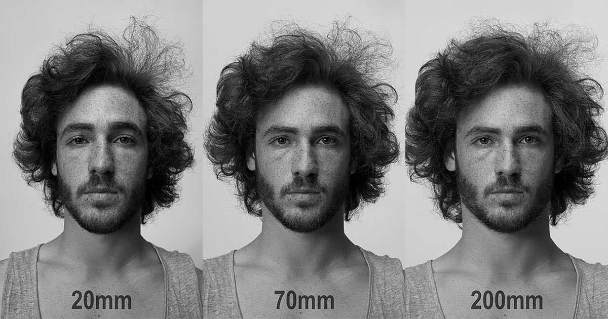
Thus, any user declaration of a class that inherits from [LocalParameterization](http://ceres-solver.org/nnls_modeling.html#costfunction|CostFunction]] or [[http://ceres-solver.org/nnls_modeling.html#localparameterization) requires the specification of Jacobians. This can get really tedious really fast, which is why Ceres offers auto-diff in the form of two alternative classes to define through templating and inheritance (see the links for details):

• AutoDiffCostFunction: A templated class that takes as an argument a user-defined "functor" class or struct implementing the residual function.
• AutoDiffLocalParameterization: A templated class that takes as an argument a user-defined "plus" class or struct implementing the $\oplus$ operator.

Small Robotics Examples with Ceres (in Python)

Ceres is a C$++$ library, and its speed is certainly dependent on programming in that language. That said, I've found it useful to use Python bindings to learn the library by doing quick experiments solving small-scale robotics problems.

Below are some examples of Ceres applied to small robotics problems of increasing complexity--they should give a sense of what the library is capable of, and perhaps even facilitate your own prototyping efforts. The Python syntax translates pretty well to C$++$, but of course the Ceres website serves as the best C$++$ API reference.

Linux Setup

If you wish to run/modify the following examples yourself, you’ll need to install these Python packages:

• numpy
  • For working with vectors and some basic linear algebra.
• matplotlib
  • For visualization.
• ceres_python_bindings$^*$
  • Third-party Python bindings for Ceres < 2.1.0. Provides the core library API discussed above.
• geometry$^*$
  • Python bindings for a C$++$ templated library that implements the chart map operations for $SO(3)$ and $SE(3)$. With this library, the $\oplus$ and $\ominus$ operators are abstracted away into the normal plus and minus operators.
• pyceres_factors$^*$
  • Python bindings for custom cost functions for Ceres that make use of the geometry package above.

$^$ These are custom Python packages that must be built from source. Follow the build instructions in each link above, then add the geometry.cpython-.so and pyceres.cpython-.so* library files to your PYTHONPATH environment variable.

If you're a [nixpkgs overlay](https://nixos.org/|Nix]] user, I maintain derivations of these packages in a [[https://github.com/goromal/anixpkgs). Following the README directions, a minimal Nix shell needed to run this tutorial can be spawned with this shell.nix file:

{ pkgs ? import <nixpkgs> {} }: # <nixpkgs> should point to overlay
let
  python-with-my-packages = pkgs.python39.withPackages (p: with p; [
    numpy
    matplotlib
    geometry
    pyceres
    pyceres_factors
  ]);
in
python-with-my-packages.env

Outline

Here's an outline of the incrementally harder problems covered in the coming sections:

Hello World

This isn't really a robotics problem--it's the Python-wrapped version of Ceres' hello world tutorial, where the goal is to minimize the cost function

$$J(x)=\frac{1}{2}(10-x)^2.$$

The code:

import PyCeres # Import the Python Bindings
import numpy as np

# The variable to solve for with its initial value.
initial_x = 5.0
x = np.array([initial_x]) # Requires the variable to be in a numpy array

# Here we create the problem as in normal Ceres
problem = PyCeres.Problem()

# Creates the CostFunction. This example uses a C++ wrapped function which 
# returns the Autodiffed cost function used in the C++ example
cost_function = PyCeres.CreateHelloWorldCostFunction()

# Add the costfunction and the parameter numpy array to the problem
problem.AddResidualBlock(cost_function, None, x) 

# Setup the solver options as in normal ceres
options=PyCeres.SolverOptions()
# Ceres enums live in PyCeres and require the enum Type
options.linear_solver_type = PyCeres.LinearSolverType.DENSE_QR
options.minimizer_progress_to_stdout = True
summary = PyCeres.Summary()
# Solve as you would normally
PyCeres.Solve(options, problem, summary)
print(summary.BriefReport() + " \n")
print( "x : " + str(initial_x) + " -> " + str(x) + "\n")

The output should look like

iter      cost      cost_change  |gradient|   |step|    tr_ratio  tr_radius  ls_iter  iter_time  total_time
   0  1.250000e+01    0.00e+00    5.00e+00   0.00e+00   0.00e+00  1.00e+04        0    6.91e-06    5.70e-05
   1  1.249750e-07    1.25e+01    5.00e-04   5.00e+00   1.00e+00  3.00e+04        1    1.79e-05    1.04e-04
   2  1.388518e-16    1.25e-07    1.67e-08   5.00e-04   1.00e+00  9.00e+04        1    3.10e-06    1.13e-04
Ceres Solver Report: Iterations: 3, Initial cost: 1.250000e+01, Final cost: 1.388518e-16, Termination: CONVERGENCE 

x : 5.0 -> [9.99999998]

1D SLAM with Range Measurements

In this simplified SLAM problem, a robot is moving along a line, obtaining noisy relative transform measurements $T$ and collecting noisy range measurements $z$ to three different landmarks. The cost function is the sum of all measurement residuals,

$$J(\hat{\boldsymbol{x}},\hat{\boldsymbol{l}})=\sum_{i=1}^8\left(\lvert\lvert T_i-\hat{T}i\rvert\rvert{\sigma_T}^2+\sum_{j=1}^3\lvert\lvert z_{i,j}-\hat{z}{i,j}\rvert\rvert{\sigma_z}^2\right),$$

for all states $\boldsymbol{x}$ and landmarks $\boldsymbol{l}$ over eight time steps. In this case, since it's in one dimension, the relative transform and range measurements are both computed simply by subtracting two numbers--no need for vector math or local parameterizations. Note the definitions of the Transform1D and Range1D factors as cost objects with provided analytic derivatives. In the future, we'll try defining factors with the help of AutoDiff.

The code:

import PyCeres as ceres
import numpy as np

##
# 1D SLAM with range measurements
##

# "Between Factor" for 1D transform measurement
class Transform1DFactor(ceres.CostFunction):
    # factor initialized with a measurement and an associated variance
    def __init__(self, z, var):
        super().__init__()
        # set size of residuals and parameters
        self.set_num_residuals(1)
        self.set_parameter_block_sizes([1,1])
        # set internal factor variables
        self.transform = z
        self.var = var

    # computes the residual and jacobian from the factor and connected state edges
    def Evaluate(self, parameters, residuals, jacobians):
        # measurement residual compares estimated vs measured transform, scaled by
        # measurement belief
        xi = parameters[0][0]
        xj = parameters[1][0]
        residuals[0] = (self.transform - (xj - xi)) / self.var

        # jacobian of the residual w.r.t. the parameters
        if jacobians != None:
            if jacobians[0] != None:
                jacobians[0][0] = 1.0 / self.var
            if jacobians[1] != None:
                jacobians[1][0] = -1.0 / self.var

        return True

class Range1DFactor(ceres.CostFunction):
    def __init__(self, z, var):
        super().__init__()
        self.set_num_residuals(1)
        self.set_parameter_block_sizes([1,1])
        self.range = z
        self.var = var

    def Evaluate(self, parameters, residuals, jacobians):
        # measurement residual compares estimated vs measured distance to a
        # specific landmark, scaled by measurement belief
        l = parameters[0][0]
        x = parameters[1][0]
        residuals[0] = (self.range - (l - x)) / self.var

        if jacobians != None:
            if jacobians[0] != None:
                jacobians[0][0] = -1.0 / self.var
            if jacobians[1] != None:
                jacobians[1][0] = 1.0 / self.var

        return True

# optimization problem
problem = ceres.Problem()

# true state positions
x = np.array([0., 1., 2., 3., 4., 5., 6., 7.]) 
# true landmark positions
l = np.array([10., 15., 13.])

# faulty landmark position beliefs
lhat = np.array([11., 12., 15.])

# simulate noisy 1D state estimates and landmark measurements that will
# be added to the problem as factors
xhat = np.array([0., 0., 0., 0., 0., 0., 0., 0.])
mu, sigma = 0.0, 1.0 # for normal distribution scalable by variance
Tvar = 1.0e-3 # variance of transform measurement noise
rvar = 1.0e-5 # variance of range measurement noise
for i in range(x.size):
    if i > 0:
        # measured relative transform in 1D 
        That = x[i] - x[i-1] + np.random.normal(mu, sigma, 1).item() * np.sqrt(Tvar)
        # propagate frontend state estimate
        xhat[i] = xhat[i-1] + That
        # add between factor to problem
        problem.AddResidualBlock(Transform1DFactor(That, Tvar), None, xhat[i-1:i], xhat[i:i+1])

    for j in range(l.size):
        # measured range from robot pose i to landmark j
        zbar = l[j] - x[i] + np.random.normal(mu, sigma, 1).item() * np.sqrt(rvar)
        # add range factor to problem
        problem.AddResidualBlock(Range1DFactor(zbar, rvar), None, lhat[j:j+1], xhat[i:i+1])

# initial error, for reference
init_error = np.linalg.norm(x - xhat) + np.linalg.norm(l - lhat)

# set solver options
options = ceres.SolverOptions()
options.max_num_iterations = 25
options.linear_solver_type = ceres.LinearSolverType.DENSE_QR
options.minimizer_progress_to_stdout = True

# solve!
summary = ceres.Summary()
ceres.Solve(options, problem, summary)

# report results
# print(summary.FullReport())
final_error = np.linalg.norm(x - xhat) + np.linalg.norm(l - lhat)
print('Total error of optimized states and landmarks: %f -> %f' % (init_error, final_error))

The output should look something similar (there's some randomness due to the noise definition) to:

iter      cost      cost_change  |gradient|   |step|    tr_ratio  tr_radius  ls_iter  iter_time  total_time
   0  5.602067e+11    0.00e+00    2.40e+11   0.00e+00   0.00e+00  1.00e+04        0    5.33e-04    6.07e-04
   1  6.610002e+05    5.60e+11    2.40e+07   3.74e+00   1.00e+00  3.00e+04        1    5.99e-04    1.25e-03
   2  6.553993e+05    5.60e+03    8.00e+02   3.74e-04   1.00e+00  9.00e+04        1    5.58e-04    1.82e-03
Total error of optimized states and landmarks: 3.793793 -> 0.014236

Rotation Averaging with Quaternions and AutoDiff

Problem Overview

This example introduces optimization over the manifold of quaternions, as well as auto-differentiation in Ceres. The cost function simply consists of the residual between a single estimated quaternion and $N$ randomly-dispersed quaternions:

$$J(\hat{\boldsymbol{q}})=\sum_{i=1}^N\lvert\lvert \boldsymbol{q}_i\ominus\hat{\boldsymbol{q}}\rvert\rvert_2^2.$$

Preliminary Class Definitions

From here on out, the derivatives get annoying enough that we will make exclusive use of AutoDiff to calculate our cost function Jacobians. Because the Python bindings don't provide helpful tools for defining an auto-differentiated cost function in Python, the local parameterization and cost function must be implemented in C$++$ and then wrapped in a Python constructor. Luckily, these C$++$ classes are already implemented for rotations (implemented on the $SO(3)$ manifold) and rigid body transformations (implemented on the $SE(3)$ manifold) in the [Python wrappers](https://github.com/goromal/ceres-factors|ceres-factors]] library with corresponding [[https://github.com/goromal/pyceres_factors). Check out the ceres-factors library to get a sense of how these classes are implemented, if you're interested.

Optimization Routine

For the main Ceres solver code, we'll actually allow for the option to not define a special LocalParameterization for the quaternion decision variable, just so we can see how it affects the solution. When no LocalParameterization is given, Ceres will assume that the parameter is just a regular vector, and so will perform operations that will inevitably make the parameter leave the manifold it's supposed to be constrained to.

The code:

import numpy as np
from geometry import SO3
import PyCeres as ceres
import PyCeresFactors as factors

##
# Rotation Averaging with Quaternions
##

# If false, will treat the quaternion decision variable as a vector
LOCAL_PARAMETERIZATION = True

# number of rotations to average over
N = 1000
# scaling factor for noisy rotations
noise_scale = 1e-2
# represent the noise as a covariance matrix for the estimator
Q = np.sqrt(noise_scale) * np.eye(3)

# true average quaternion
q = SO3.random()

# initial vector guess for average quaternion
xhat = SO3.identity().array()

# optimization problem
problem = ceres.Problem()

# if using local parameterization, add it to the problem
if LOCAL_PARAMETERIZATION:
    problem.AddParameterBlock(xhat, 4, factors.SO3Parameterization())

# create noisy rotations around the true average and add to problem as 
# measurement residuals
for i in range(N):
    sample = (q + np.random.random(3) * noise_scale).array()
    problem.AddResidualBlock(factors.SO3Factor(sample, Q),
                             None,
                             xhat)

# set solver options
options = ceres.SolverOptions()
options.max_num_iterations = 25
options.linear_solver_type = ceres.LinearSolverType.DENSE_QR
options.minimizer_progress_to_stdout = True

# solve!
summary = ceres.Summary()
ceres.Solve(options, problem, summary)

# report results
q_hat = SO3(xhat)
print('q:', q)
print('q_hat:', q_hat)
if not LOCAL_PARAMETERIZATION:
    print('q_hat (normalized):', q_hat.normalized())

Results

With LOCAL_PARAMETERIZATION set to True, the output will look something like this:

iter      cost      cost_change  |gradient|   |step|    tr_ratio  tr_radius  ls_iter  iter_time  total_time
   0  1.613744e+05    0.00e+00    6.62e-01   0.00e+00   0.00e+00  1.00e+04        0    2.29e-04    3.36e-04
   1  1.262180e+00    1.61e+05    1.03e+00   8.68e-01   1.00e+00  3.00e+04        1    3.84e-04    7.44e-04
   2  1.259806e+00    2.37e-03    3.07e-04   1.09e-04   1.00e+00  9.00e+04        1    3.46e-04    1.10e-03
q: SO(3): [ 0.625178, -0.194097i, 0.520264j, 0.548456k]
q_hat: SO(3): [ 0.622974, -0.192598i, 0.523643j, 0.548277k]

If LOCAL_PARAMETERIZATION is set to False, then an output similar to the following will be shown. Note that quaternion normalization is needed to actually return a valid answer. It even takes more iterations to converge!

iter      cost      cost_change  |gradient|   |step|    tr_ratio  tr_radius  ls_iter  iter_time  total_time
   0  1.613945e+05    0.00e+00    2.52e+05   0.00e+00   0.00e+00  1.00e+04        0    1.97e-04    3.16e-04
   1  5.546311e+03    1.56e+05    3.31e+04   8.98e-01   9.66e-01  3.00e+04        1    4.31e-04    7.74e-04
   2  1.055270e+01    5.54e+03    1.65e+03   2.33e-01   9.98e-01  9.00e+04        1    3.39e-04    1.12e-03
   3  1.238904e+00    9.31e+00    8.84e-01   8.88e-03   1.00e+00  2.70e+05        1    3.20e-04    1.45e-03
   4  1.238901e+00    2.69e-06    4.85e-06   4.78e-06   1.00e+00  8.10e+05        1    3.10e-04    1.76e-03
q: SO(3): [ 0.625178, -0.194097i, 0.520264j, 0.548456k]
q_hat: SO(3): [ 0.808827, -0.250154i, 0.680017j, 0.711829k]
q_hat (normalized): SO(3): [ 0.622930, -0.192660i, 0.523726j, 0.548226k]

Pose Graph SLAM

Problem Overview

The pose graph SLAM problem aims to minimize the measurement error between measured and actual relative poses:

$$J=\sum_{(i,j)\in\mathcal{E}}\lvert\lvert \hat{\boldsymbol{R}}{j}\ominus\hat{\boldsymbol{R}}{i}\boldsymbol{R}{ij}\rvert\rvert{F}^{2}+\lvert\lvert \hat{\boldsymbol{t}}{j}-\hat{\boldsymbol{t}}{i}-\hat{\boldsymbol{R}}{i}\boldsymbol{t}{ij}\rvert\rvert_{2}^{2},$$

where the edges $\mathcal{E}$ in the pose graph encompass both odometry and loop closure relative pose measurements. With $\boldsymbol{T}\in SE(3)$ and adding in covariance matrix weighting, the above can be re-written concisely as

$$J=\sum_{(i,j)\in\mathcal{E}}\lvert\lvert \left(\hat{\boldsymbol{T}}{i}^{-1}\hat{\boldsymbol{T}}j\right)\ominus\boldsymbol{T}{ij}\rvert\rvert{\boldsymbol{\Sigma}}^{2}.$$

/*#### Preliminary Class Definitions

To perform full-on pose graph optimization with Ceres, the following definitions are needed:

• An $SE(3)$ group implementation that overloads the +/- operators with $\oplus$/$\ominus$. We will use the SE3 class from Sophus.
• An AutoDiff local parameterization for the $SE(3)$ group, since Ceres doesn't ship with one.
• An AutoDiff cost function/factor for the residual obtained by subtracting a measured relative $SE(3)$ transform and the current estimated relative $SE(3)$ transform, i.e., an edge in the pose graph.

First, some convenience functions for converting to/from the SE3 type:

// cSE3 conversion functions: to/from pointer/vector
template<typename T>
void cSE3convert(const T* data, Sophus::SE3<T>& X) {
  X = Sophus::SE3<T>(Eigen::Quaternion<T>(data+3),
                     Eigen::Map<const Eigen::Matrix<T,3,1>>(data));
}
template<typename T>
void cSE3convert(const Eigen::Matrix<T,7,1> &Xvec, Sophus::SE3<T>& X) {
  X = Sophus::SE3<T>(Eigen::Quaternion<T>(Xvec.data()+3),
                     Eigen::Map<const Eigen::Matrix<T,3,1>>(Xvec.data()));
}
template<typename T>
void cSE3convert(const Sophus::SE3<T>& X, Eigen::Matrix<T,7,1> &Xvec) {
  Xvec.template block<3,1>(0,0) = Eigen::Matrix<T,3,1>(X.translation().data());
  Xvec.template block<4,1>(3,0) = Eigen::Matrix<T,4,1>(X.so3().data());
}

The definition for (2) follows, which functions a lot like Ceres' built-in EigenQuaternionLocalParameterization class--just with an added translation component:

* AutoDiff local parameterization for the compact SE3 pose [t q] object. 
* The boxplus operator informs Ceres how the manifold evolves and also  
* allows for the calculation of derivatives.
struct cSE3Plus {
  * boxplus operator for both doubles and jets
  template<typename T>
  bool operator()(const T* x, const T* delta, T* x_plus_delta) const
  {
    * capture argument memory
    Sophus::SE3<T> X;
    cSE3convert(x, X);
    Eigen::Map<const Eigen::Matrix<T, 6, 1>> dX(delta);
    Eigen::Map<Eigen::Matrix<T, 7, 1>>       Yvec(x_plus_delta);

    * increment pose using the exponential map
    Sophus::SE3<T> Exp_dX = Sophus::SE3<T>::exp(dX);
    Sophus::SE3<T> Y = X * Exp_dX;

    * assign SE3 coefficients to compact vector
    Eigen::Matrix<T,7,1> YvecCoef;
    cSE3convert(Y, YvecCoef);
    Yvec = YvecCoef;

    return true;
  }
  
  * local parameterization generator--ONLY FOR PYTHON WRAPPER
  static ceres::LocalParameterization *Create() {
    return new ceres::AutoDiffLocalParameterization<cSE3Plus,
                                                    7,
                                                    6>(new cSE3Plus);
  }
};

The definition for (3) also looks a lot like the Quaternion-based cost function implemented for rotation averaging, again with an added translation component. Also note the addition of the inverse covariance matrix for weighting residuals:

* AutoDiff cost function (factor) for the difference between a measured 3D
* relative transform, Xij = (tij_, qij_), and the relative transform between two  
* estimated poses, Xi_hat and Xj_hat. Weighted by measurement covariance, Qij_.
class cSE3Functor
{
public:
EIGEN_MAKE_ALIGNED_OPERATOR_NEW
  * store measured relative pose and inverted covariance matrix
  cSE3Functor(Eigen::Matrix<double,7,1> &Xij_vec, Eigen::Matrix<double,6,6> &Qij)
  {
    Sophus::SE3<double> Xij;
    cSE3convert(Xij_vec, Xij);
    Xij_inv_ = Xij.inverse();
    Qij_inv_ = Qij.inverse();
  }

  * templated residual definition for both doubles and jets
  * basically a weighted implementation of boxminus using Eigen templated types
  template<typename T>
  bool operator()(const T* _Xi_hat, const T* _Xj_hat, T* _res) const
  {
    * assign memory to usable objects
    Sophus::SE3<T> Xi_hat, Xj_hat;
    cSE3convert(_Xi_hat, Xi_hat);
    cSE3convert(_Xj_hat, Xj_hat);
    Eigen::Map<Eigen::Matrix<T,6,1>> r(_res);

    * compute current estimated relative pose
    const Sophus::SE3<T> Xij_hat = Xi_hat.inverse() * Xj_hat;

    * compute residual via boxminus (i.e., the logarithmic map of the error pose)
    * weight with inverse covariance
    r = Qij_inv_.cast<T>() * (Xij_inv_.cast<T>() * Xij_hat).log();        

    return true;
  }

  // cost function generator--ONLY FOR PYTHON WRAPPER
  static ceres::CostFunction *Create(Eigen::Matrix<double,7,1> &Xij, Eigen::Matrix<double,6,6> &Qij) {
    return new ceres::AutoDiffCostFunction<cSE3Functor,
                                           6,
                                           7,
                                           7>(new cSE3Functor(Xij, Qij));
  }

private:
  Sophus::SE3<double> Xij_inv_;
  Eigen::Matrix<double,6,6> Qij_inv_;
};

Note that both (2) and (3) take advantage of Sophus' implemented chart operations for $SE(3)$. Further, auto-differentiation is possible because of Sophus' templated classes, modeled after Eigen's templated classes.*/

/Note that because we defined our Transform3D object in Python, we ended up implementing both $\oplus$ and $\ominus$ twice--once in the class definition and once in the parameterization and factor definitions. Maybe implementing them in both languages was informative, but a smarter thing to do in the future would be to define the base Lie Group class in C$++$ (or even utilize some pre-written classes like the ones from the Sophus library) and then utilize its overloaded operator directly for shorter parameterization and factor definitions. Finally, if you paid very close attention, you'll notice that I made a slight but important error in my $\oplus$ and $\ominus$ implementations by not adding a rotation matrix term to the translation vector operations. Again, an error that could be avoided by using classes provided by other libraries! However, as we'll see in the optimization routine, because my $SE(3)$ implementation was consistent throughout, we can still extract a minimizing trajectory. I guess we can pretend that relative translation measurements were all given in the global frame and call it good.../

Optimization Routine

Putting everything together, we simulate a simple robot moving in a circle, obtaining noisy odometry and loop closure measurements as it moves along. These noisy measurements are used to formulate and solve the pose graph optimization problem:

import numpy as np
import matplotlib.pyplot as plt
from geometry import SE3
import PyCeres as ceres
import PyCeresFactors as factors

##
# Pose Graph SLAM
##

# odom, loop closure covariances (linear, angular)
odom_cov_vals = (0.5, 0.01)
lc_cov_vals = (0.001, 0.0001)

# simulation parameters
num_steps = 50
num_lc = 12 # number of loop closures to insert

# delta pose/odometry between successive nodes in graph (tangent space representation as a local perturbation)
dx = np.array([1.,0.,0.,0.,0.,0.1])

# odometry covariance
odom_cov = np.eye(6)
odom_cov[:3,:3] *= odom_cov_vals[0] # delta translation noise
odom_cov[3:,3:] *= odom_cov_vals[1] # delta rotation noise
odom_cov_sqrt = np.linalg.cholesky(odom_cov)

# loop closure covariance
lc_cov = np.eye(6)
lc_cov[:3,:3] *= lc_cov_vals[0] # relative translation noise
lc_cov[3:,3:] *= lc_cov_vals[1] # relative rotation noise
lc_cov_sqrt = np.linalg.cholesky(lc_cov)

# truth/estimate buffers
x = list()
xhat = list() # in Python, need to keep parameter arrays separate to prevent memory aliasing

# determine which pose indices will have loop closures between them
loop_closures = list()
for l in range(num_lc):
    i = np.random.randint(low=0, high=num_steps-1)
    j = np.random.randint(low=0, high=num_steps-2)
    if j == i:
        j = num_steps-1
    loop_closures.append((i,j))

# optimization problem
problem = ceres.Problem()

# create odometry measurements
for k in range(num_steps):
    if k == 0:
        # starting pose
        xhat.append(SE3.identity().array())
        x.append(SE3.identity().array())

        # add (fixed) prior to the graph
        problem.AddParameterBlock(xhat[k], 7, factors.SE3Parameterization())
        problem.SetParameterBlockConstant(xhat[k])
    else:
        # time step endpoints
        i = k-1
        j = k

        # simulate system
        x.append((SE3(x[i]) + dx).array())

        # create noisy front-end measurement (constrained to the horizontal plane)
        dx_noise = odom_cov_sqrt.dot(np.random.normal(np.zeros(6), np.ones(6), (6,)))
        dx_noise[2] = dx_noise[3] = dx_noise[4] = 0.
        dxhat = SE3.Exp(dx + dx_noise)
        xhat.append((SE3(xhat[i]) * dxhat).array())

        # add relative measurement to the problem as a between factor (with appropriate parameterization)
        problem.AddParameterBlock(xhat[j], 7, factors.SE3Parameterization())
        problem.AddResidualBlock(factors.RelSE3Factor(dxhat.array(), odom_cov), None, xhat[i], xhat[j])

# create loop closure measurements
for l in range(num_lc):
    i = loop_closures[l][0]
    j = loop_closures[l][1]

    # noise-less loop closure measurement
    xi = SE3(x[i])
    xj = SE3(x[j])
    xij = xi.inverse() * xj

    # add noise to loop closure measurement (constrained to the horizontal plane)
    dx_noise = lc_cov_sqrt.dot(np.random.normal(np.zeros(6), np.ones(6), (6,)))
    dx_noise[2] = dx_noise[3] = dx_noise[4] = 0.
    dx_meas = xij + dx_noise

    # add relative measurement to the problem as a between factor
    problem.AddResidualBlock(factors.RelSE3Factor(dx_meas.array(), lc_cov), None, xhat[i], xhat[j])

# initial error, for reference
prev_err = 0.
x1_true = list()
x2_true = list()
x1_init = list()
x2_init = list()
for k in range(num_steps):
    prev_err += 1.0/6.0*np.linalg.norm(x[k] - xhat[k])**2
    x1_true.append(x[k][0])
    x2_true.append(x[k][1])
    x1_init.append(xhat[k][0])
    x2_init.append(xhat[k][1])
prev_err /= num_steps

# set solver options
options = ceres.SolverOptions()
options.max_num_iterations = 25
options.linear_solver_type = ceres.LinearSolverType.SPARSE_NORMAL_CHOLESKY
options.minimizer_progress_to_stdout = True

# solve!
summary = ceres.Summary()
ceres.Solve(options, problem, summary)

# report results
post_err = 0.
x1_final = list()
x2_final = list()
for k in range(num_steps):
    post_err += 1.0/6.0*np.linalg.norm(x[k] - xhat[k])**2
    x1_final.append(xhat[k][0])
    x2_final.append(xhat[k][1])
post_err /= num_steps
print('Average error of optimized poses: %f -> %f' % (prev_err, post_err))

# plot results
fig, ax = plt.subplots()
ax.plot(x1_true, x2_true, color='black', label='truth')
ax.plot(x1_init, x2_init, color='red', label='xhat_0')
ax.plot(x1_final, x2_final, color='blue', label='xhat_f')
ax.set_title('Pose Graph Optimization Example')
ax.set_xlabel('x (m)')
ax.set_ylabel('y (m)')
ax.legend()
ax.grid()
plt.show()

Viewing the results from the command line will give something like this:

iter      cost      cost_change  |gradient|   |step|    tr_ratio  tr_radius  ls_iter  iter_time  total_time
   0  2.643133e+09    0.00e+00    1.91e+00   0.00e+00   0.00e+00  1.00e+04        0    1.62e-03    2.14e-03
   1  2.872315e+08    2.36e+09    2.86e+02   1.03e+02   8.95e-01  1.97e+04        1    1.98e-03    4.16e-03
   2  9.150302e+05    2.86e+08    4.99e+02   3.11e+01   9.97e-01  5.90e+04        1    1.51e-03    5.69e-03
   3  1.600187e+04    8.99e+05    9.67e+01   5.52e+00   1.00e+00  1.77e+05        1    1.59e-03    7.29e-03
   4  1.536517e+04    6.37e+02    2.95e+01   5.41e+00   1.00e+00  5.31e+05        1    1.48e-03    8.78e-03
   5  1.530853e+04    5.66e+01    3.66e+00   3.38e+00   1.00e+00  1.59e+06        1    1.39e-03    1.02e-02
   6  1.530598e+04    2.55e+00    6.84e-01   8.33e-01   1.00e+00  4.78e+06        1    1.33e-03    1.15e-02
   7  1.530597e+04    1.73e-02    4.78e-02   7.25e-02   1.00e+00  1.43e+07        1    1.31e-03    1.28e-02
Average error of optimized poses: 31.432182 -> 0.040357

and a quick plot of the trajectories for several covariance and simulation parameter combinations gives a more intuitive evaluative measure:

Pose Graph SLAM with Range Measurements

Problem Overview

For this final example, we add point-to-point range measurements for random pose pairs along the trajectory:

$$J=\sum_{(i,j)\in\mathcal{E}}\lvert\lvert \left(\hat{\boldsymbol{T}}{i}^{-1}\hat{\boldsymbol{T}}j\right)\ominus\boldsymbol{T}{ij}\rvert\rvert{\boldsymbol{\Sigma}}^{2}+\lvert\lvert \lvert\lvert \hat{\boldsymbol{t}}{j}-\hat{\boldsymbol{t}}{i}\rvert\rvert_2-r_{ij}\rvert\rvert_{\boldsymbol{\Sigma}}^2,$$

which isn't very realistic, but can be informative about the feasibility of a larger problem of utilizing inter-agent range measurements in a multi-agent SLAM scenario to reduce drift without relying heavily on inter-agent loop closure detection and communication. The PyCeresFactors.RangeFactor function wrapper implements this custom cost function.

Optimization Routine

The Python code is very similar to the pure pose graph problem--just with added range measurement simulation and corresponding range factors:

import numpy as np
import matplotlib.pyplot as plt
from geometry import SE3
import PyCeres as ceres
import PyCeresFactors as factors

##
# Pose Graph SLAM with Range Measurements
##

# odom, loop closure covariances (linear, angular)
odom_cov_vals = (0.5, 0.01)
lc_cov_vals = (0.001, 0.0001)

# range variance
range_cov = 0.01

# simulation parameters
num_steps = 50
num_lc = 12
num_range = 12

# delta pose/odometry between successive nodes in graph (tangent space representation as a local perturbation)
dx = np.array([1.,0.,0.,0.,0.,0.1])

# odometry covariance
odom_cov = np.eye(6)
odom_cov[:3,:3] *= odom_cov_vals[0] # delta translation noise
odom_cov[3:,3:] *= odom_cov_vals[1] # delta rotation noise
odom_cov_sqrt = np.linalg.cholesky(odom_cov)

# loop closure covariance
lc_cov = np.eye(6)
lc_cov[:3,:3] *= lc_cov_vals[0] # relative translation noise
lc_cov[3:,3:] *= lc_cov_vals[1] # relative rotation noise
lc_cov_sqrt = np.linalg.cholesky(lc_cov)

# range covariance
range_cov_sqrt = np.sqrt(range_cov)

# truth/estimate buffers
x = list()
xhat = list() # in Python, need to keep parameter arrays separate to prevent memory aliasing

# determine which pose indices will have loop closures between them
loop_closures = list()
for l in range(num_lc):
    i = np.random.randint(low=0, high=num_steps-1)
    j = np.random.randint(low=0, high=num_steps-2)
    if j == i:
        j = num_steps-1
    loop_closures.append((i,j))

# determine which pose indices will have range measurements between them
range_measurements = list()
for l in range(num_range):
    i = np.random.randint(low=0, high=num_steps-1)
    j = np.random.randint(low=0, high=num_steps-2)
    if j == i:
        j = num_steps-1
    range_measurements.append((i,j))

# optimization problem
problem = ceres.Problem()

# create odometry measurements
for k in range(num_steps):
    if k == 0:
        # starting pose
        xhat.append(SE3.identity().array())
        x.append(SE3.identity().array())

        # add (fixed) prior to the graph
        problem.AddParameterBlock(xhat[k], 7, factors.SE3Parameterization())
        problem.SetParameterBlockConstant(xhat[k])
    else:
        # time step endpoints
        i = k-1
        j = k

        # simulate system
        x.append((SE3(x[i]) + dx).array())

        # create noisy front-end measurement (constrained to the horizontal plane)
        dx_noise = odom_cov_sqrt.dot(np.random.normal(np.zeros(6), np.ones(6), (6,)))
        dx_noise[2] = dx_noise[3] = dx_noise[4] = 0.
        dxhat = SE3.Exp(dx + dx_noise)
        xhat.append((SE3(xhat[i]) * dxhat).array())

        # add relative measurement to the problem as a between factor (with appropriate parameterization)
        problem.AddParameterBlock(xhat[j], 7, factors.SE3Parameterization())
        problem.AddResidualBlock(factors.RelSE3Factor(dxhat.array(), odom_cov), None, xhat[i], xhat[j])

# create loop closure measurements
for l in range(num_lc):
    i = loop_closures[l][0]
    j = loop_closures[l][1]

    # noise-less loop closure measurement
    xi = SE3(x[i])
    xj = SE3(x[j])
    xij = xi.inverse() * xj

    # add noise to loop closure measurement (constrained to the horizontal plane)
    dx_noise = lc_cov_sqrt.dot(np.random.normal(np.zeros(6), np.ones(6), (6,)))
    dx_noise[2] = dx_noise[3] = dx_noise[4] = 0.
    dx_meas = xij + dx_noise

    # add relative measurement to the problem as a between factor
    problem.AddResidualBlock(factors.RelSE3Factor(dx_meas.array(), lc_cov), None, xhat[i], xhat[j])

# create range measurements
for r in range(num_range):
    i = range_measurements[r][0]
    j = range_measurements[r][1]

    # noise-less range measurement
    ti = x[i][:3]
    tj = x[j][:3]
    rij = np.linalg.norm(tj - ti)

    # add noise to range measurement
    r_noise = range_cov_sqrt * np.random.normal(0.0, 1.0, 1).item()

    # add range measurement to the problem as a range factor
    problem.AddResidualBlock(factors.RangeFactor(rij, range_cov), None, xhat[i], xhat[j])

# initial error, for reference
prev_err = 0.
x1_true = list()
x2_true = list()
x1_init = list()
x2_init = list()
for k in range(num_steps):
    prev_err += 1.0/6.0*np.linalg.norm(x[k] - xhat[k])**2
    x1_true.append(x[k][0])
    x2_true.append(x[k][1])
    x1_init.append(xhat[k][0])
    x2_init.append(xhat[k][1])
prev_err /= num_steps

# set solver options
options = ceres.SolverOptions()
options.max_num_iterations = 25
options.linear_solver_type = ceres.LinearSolverType.SPARSE_NORMAL_CHOLESKY
options.minimizer_progress_to_stdout = True

# solve!
summary = ceres.Summary()
ceres.Solve(options, problem, summary)

# report results
post_err = 0.
x1_final = list()
x2_final = list()
for k in range(num_steps):
    post_err += 1.0/6.0*np.linalg.norm(x[k] - xhat[k])**2
    x1_final.append(xhat[k][0])
    x2_final.append(xhat[k][1])
post_err /= num_steps
print('Average error of optimized poses: %f -> %f' % (prev_err, post_err))

# plot results
fig, ax = plt.subplots()
ax.plot(x1_true, x2_true, color='black', label='truth')
ax.plot(x1_init, x2_init, color='red', label='xhat_0')
ax.plot(x1_final, x2_final, color='blue', label='xhat_f')
ax.set_title('PGO + Range Example')
ax.set_xlabel('x (m)')
ax.set_ylabel('y (m)')
ax.legend()
ax.grid()
plt.show()

Results

Some sample output as a sanity check:

iter      cost      cost_change  |gradient|   |step|    tr_ratio  tr_radius  ls_iter  iter_time  total_time
   0  2.189067e+08    0.00e+00    5.24e+04   0.00e+00   0.00e+00  1.00e+04        0    7.62e-04    1.10e-03
   1  1.157768e+06    2.18e+08    6.49e+03   1.56e+01   9.95e-01  3.00e+04        1    1.29e-03    2.42e-03
   2  2.895435e+03    1.15e+06    2.23e+03   3.65e+00   9.98e-01  9.00e+04        1    1.19e-03    3.62e-03
   3  9.127433e+02    1.98e+03    2.32e+02   2.79e+00   9.92e-01  2.70e+05        1    1.21e-03    4.85e-03
   4  8.610937e+02    5.16e+01    2.89e+02   3.53e+00   7.24e-01  2.97e+05        1    1.19e-03    6.05e-03
   5  8.271397e+02    3.40e+01    8.19e+01   2.52e+00   9.70e-01  8.90e+05        1    1.17e-03    7.23e-03
   6  8.133719e+02    1.38e+01    8.09e+01   4.37e+00   9.41e-01  2.67e+06        1    1.18e-03    8.43e-03
   7  8.049370e+02    8.43e+00    1.10e+02   5.30e+00   9.18e-01  6.42e+06        1    1.17e-03    9.60e-03
   8  8.025589e+02    2.38e+00    4.76e+01   2.99e+00   9.59e-01  1.93e+07        1    1.32e-03    1.09e-02
   9  8.023315e+02    2.27e-01    5.95e+00   8.69e-01   1.00e+00  5.78e+07        1    1.82e-03    1.28e-02
  10  8.023281e+02    3.40e-03    1.90e-01   1.04e-01   1.02e+00  1.73e+08        1    1.54e-03    1.43e-02
Average error of optimized poses: 2.014479 -> 0.186329

And some plots, which are more interesting to look at. It looks like range measurements can indeed help keep front-end drift under control, despite the fact that they only provide 1D information embedded in 3D space!

Additional Examples

• [[public:autonomy:implementation:opt-libs:ceres-rangebearing]]

2D Range-Bearing Landmark Resolution with Ceres

FIXME UNDER CONSTRUCTION FIXME

High-level problem description: A moving vehicle confined to the 2D plane is equipped with a range-bearing device that is giving noisy 2D range and bearing measurements pointing to a static landmark at regular intervals. The bearing error in the measurement can be thought of as a product of noise as well as a steady bias, whereas the range measurement is just noisy. The goal is to incrementally collapse uncertainty about where the static landmark is by moving the vehicle around and continually collecting noisy and biased measurements.

This article will lay out some approximating equations to solve this problem and provide a Python script to test out the solution together with some high-level observations.

Prerequisite Readings

• Math context: [[public:autonomy:search-optimization:least-squares]]
• Solver context: [[public:autonomy:implementation:opt-libs:ceres]]

Running the Python Demo

If you wish to run/modify the demo yourself, you’ll need to install these Python packages:

• numpy
  • For working with vectors and some basic linear algebra.
• matplotlib
  • For visualization.
• ceres_python_bindings$^*$
  • Third-party Python bindings for Ceres < 2.1.0. Provides the core library API discussed above.
• geometry$^*$
  • Python bindings for a C$++$ templated library that implements the chart map operations for $SO(3)$ and $SE(3)$. With this library, the $\oplus$ and $\ominus$ operators are abstracted away into the normal plus and minus operators.
• pyceres_factors$^*$
  • Python bindings for custom cost functions for Ceres that make use of the geometry package above.

$^$ These are custom Python packages that must be built from source. Follow the build instructions in each link above, then add the geometry.cpython-.so and pyceres.cpython-.so* library files to your PYTHONPATH environment variable.

If you're a [overlay documentation](https://nixos.org/|Nix]] user, I maintain derivations of these packages in a [[https://github.com/goromal/anixpkgs|nixpkgs overlay]]. Following the [[https://goromal.github.io/anixpkgs/intro.html#accessing-the-packages-using-shellnix), a minimal Nix shell needed to run this demo can be spawned with this shell.nix file:

...

The three reference frames in the problem definition (see Fig. 1) are:

• The static world frame $W$
• The moving vehicle frame $B$
• The sensor frame $S$, defined for convenience as having the x-axis aligned with the detected bearing measurement.

...

Figure 1: Reference frames and uncertainty models for the range-bearing landmark localization problem. When expressed in the sensor ($S$) frame, the measurement covariance can be approximated as a diagonal matrix $\mathbf{\Sigma}^S$, though the true uncertainty distribution $\mathbf{\mathcal{U}}^S$ is a Gaussian over the $SE(2)$ manifold.

FIXME explain $\mathbf{R}_S^W$

$$\mathbf{\Sigma}^S\approx\begin{bmatrix}\sigma_d^2 & 0\0 & \left(d\sigma_{\theta}\right)^2\end{bmatrix}.$$

...

$$\mathbf{\Sigma}^W\approx\mathbf{R}_S^W\mathbf{\Sigma}^S\left(\mathbf{R}_S^W\right)^\top.$$

This measurement covariance is associated with a world-frame range-bearing measurement...

$$\mathbf{b}^W\triangleq\mathbf{R}_S^W\begin{bmatrix}d\0\end{bmatrix}.$$

...

$$\mathbf{l}^W=\mathbf{p}^W_{B/W}+\tilde{\mathbf{R}}\mathbf{b}^W.$$

...

Figure 2: Successive range-bearing measurements of a static landmark from a moving vehicle frame.

...

$$\mathbf{r}_k=\left(\mathbf{\Sigma}_k^W\right)^{-1/2}\left(\mathbf{b}k^W-\tilde{\mathbf{R}}^\top\left(\mathbf{l}^W-\mathbf{p}{B/W,k}^W\right)\right).$$

The residual implementation in C$++$ (called RangeBearing2DFactor) can be found in the ceres-factors source code (which the Python package used in this demo wraps). At each time step $k$, a factor is constructed and added to the graph from

• Measurement $d_k$ with associated standard deviation $\sigma_d$
• Measurement $\mathbf{R}{S,k}^B$ with associated standard deviation $\sigma{\theta}$ (assumed to be statically biased by an unknown mount calibration error $\tilde{\mathbf{R}}$)
• The estimated vehicle position $\mathbf{p}_{B/W,k}^W$
• The estimated vehicle orientation $\mathbf{R}_{B,k}^W$

from which the residual equation is computed using the preceding equations in this article.

Solution

...

Search and Optimization

• Least-Squares Optimization
• Nonlinear Optimization
• Optimization Over Lie Groups

Least-Squares Optimization

Why The 2-Norm?

The 2-norm, or \(\lvert\lvert\cdot\rvert\rvert_2\), is advantageous as a cost function for a number of reasons, including the following:

• It often coincides with a useful physical interpretation (e.g., energy, power).
• It is induced by the inner product \(\langle\cdot,\cdot\rangle\) operator((Inner product-induced norms expand outwards like n-dimensional spheres which, as they expand, come to touch vector spaces (i.e., "flat" spaces) at exactly one location, implying exactly one optimal solution. Hence their convexity when bounded by linear constraints (since the linear constraints provide the "flat" space).)).

A least-squares problem is, by definition, any optimization problem whose cost function is a 2-norm of some generalized residual function, \(r(x)\). Whether \(r(x)\) is linear or not((The residual equation is sometimes expressed as a constraint instead of in the cost function (rendering the cost function somewhat trivial), but usually not; both linear and nonlinear least-squares problems are generally considered to be a special case of unconstrained nonlinear optimization problems, for example.)) will completely affect how the problem is approached and solved.

Linear

Despite their name, linear least-squares problems are a subset of general unconstrained nonlinear optimization problems because of the nonlinear 2-norm operator. They're also referred to as quadratic programs. Their general form is

$$\min_x||r(x)||_2=\min_x||Ax-b||_2^2$$

with \(A\in \mathbb{R}^{m\times n}\). Optionally, a weighting matrix \(Q\) can be used:

$$\min_xr^TQr=\min_x||Q^{1/2}(Ax-b)||_2^2.$$

Solution Methods

Because this is an unconstrained nonlinear problem, we could just use some greedy search method like steepest descent, where \(F(x)=<r(x),r(x)>=(Ax-b)^T(Ax-b)\) and \(g(x)=2A^T(Ax-b)\). However, we can and should take advantage of the fact that the cost function is induced by the inner product and that the residual function is describable using vector spaces in order to derive an analytical solution. After all, what linear least squares is really asking is what is the best \(x^{*}\) such that \(Ax^{*}\) is as close to \(b\) as possible, even if \(b\) is outside of the span of \(A\). The general solution to this problem utilizes the Moore-Penrose pseudoinverse of \(A\) (assuming full row rank):

$$x^*=A^\dagger b,$$

where the pseudoinverse is defined as

• \(m>n\): \(A^\dagger=(A^TA)^{-1}A^T\)
  • Known as the left inverse (\(A^\dagger A=I\)), and exists when \(A\) is "tall," which will most likely be the case in learning problems, where you have linearly independent columns due to having more data points than variables. In this case, \(A^TA>0\) is positive definite.
• \(m=n\): \(A^\dagger=A^{-1}\)
  • The trivial case--doesn't happen very often
• \(m < n\): \(A^\dagger=A^T(AA^T)^{-1}\)
  • Known as the right inverse (\(AA^\dagger=I\)), and exists when \(A\) is "fat," which usually shows up in high- or infinite-dimensional least-squares minimization problems (like optimal control) where you have far more variables than data points. In this case, \(x^{*}\) is simply the \(x\) with the shortest 2-norm that satisfies \(Ax=b\).

Assuming that we want to calculate \(x^{*}\) with the left inverse, how to do so efficiently? Here are two methods:

Cholesky Decomposition Method

Assuming \(A^TA>0\) (again, given with the left inverse),

• Find lower triangular \(L\) such that \(A^TA=LL^T\) (Cholesky decomposition)
• Use \(Ly=A^Tb\) to obtain \(y\)
• Use \(L^Tx^*=y\) to obtain \(x^{*}\).

Faster than QR.

QR Decomposition Method

• Find \(Q\in \mathbb{R}^{n\times n},~Q^TQ=I\) and upper triangular \(R\in\mathbb{R}^{n\times n}\) such that \(A^TA=QR\) (QR decomposition)
• Solve \(Rx^*=Q^TA^Tb\) via back substitution.

More numerically stable than Cholesky.

Application to Estimation

Here, we focus on estimating quantities that don't evolve according to some modeled dynamics (unlike the Kalman Filter), so either a lot of measurements are going to help you estimate one static quantity or you are going to be trying to estimate a changing quantity at repeated snapshots, unable to take advantage of previous knowledge((There are least-squares-based estimation algorithms that also take advantage of previous solutions by using clever numerical tricks like exploiting the sparsity that shows up in SLAM problems as with incremental smoothing.)).

Problem Statement: Estimate \(\hat{x}\) (with a prior estimate \(x_0\) covariance \(Q_0\)) when the differentiable, linear measurement model is

$$y=Hx+v,~~v\sim \mathcal{N}(0,R)$$

Consider that the conditional probability density of a measurement given the state is expressed as

$$f(y|x)=\frac{1}{\alpha}e^{-\frac{1}{2}(y-Hx)^TR^{-1}(y-Hx)}$$

Thus, to get the maximum likelihood estimation of \(x\), we need to minimize the measurement error term in the exponential:

$$J=\frac{1}{2}(y-Hx)^TR^{-1}(y-Hx)$$

Or, if we’re adding a measurement update to a prior belief \(x_0\) with covariance \(Q_0\) to obtain the posterior with mean \(\hat{x}\) and covariance \(Q_1\):

$$J=\frac{1}{2}(\hat{x}-x_0)^TQ_0^{-1}(\hat{x}-x_0)+\frac{1}{2}(y-H\hat{x})^TR^{-1}(y-H\hat{x})$$

We can analytically minimize this cost function because of the linear measurement model by setting \(\frac{\partial J}{\partial \hat{x}}=0\):

$$\hat{x}=x_0+Q_1H^TR^{-1}(y-Hx_0),~Q_1=(Q_0^{-1}+H^TR^{-1}H)^{-1}$$

Note that if there were just the measurement without the prior in the cost function, differentiating and setting to zero like before would yield

$$\hat{x}=(H^TR^{-1}H)^{-1}H^TR^{-1}y=(R^{-1/2}H)^{-L}R^{-1/2}y$$

which, of course, is the weighted (by information/certainty, or inverse covariance) least squares solution to minimizing \(R^{-1/2}(y-H\hat{x})\). This makes sense, since the least squares cost function of the residual that’s linear in \(x\) (whether it’s a linear measurement model or matching the values of a polynomial that’s linear in the coefficient or parameter vector) is always minimized by projecting the observed measurement vector (or stack of measurement vectors) \(y\) (or, in this case, the scaled measurement vector \(R^{-1/2}y\)) from somewhere in the left null space onto the column space of whatever the (tall) linear operator \(H\) (or, in this weighted case, \(R^{-1/2}H\)) represents as an operator on \(x\) via the left Moore-Penrose pseudoinverse as expressed above.

So, the optimal \(\hat{x}\) is the one that makes the residual \(y-H\hat{x}=y-\hat{y}\) orthogonal to the column space or span of \(H\). Intuitively, when the goal is to minimize the variance of \(\hat{x}\), this occurs when all possible estimate information has been extracted from the measurements:

$$\tilde{x}\perp y \iff \tilde{x} \perp \hat{x} \iff E[\tilde{x}y^T]=0$$

where the equivalence comes from the fact that with linear estimators, the estimate is a linear combination of the measurements. The intuition makes sense when you think about the orthogonal projection theorem applied to regular vectors. Thus, an optimal linear estimator must satisfy the above relations.

Nonlinear

Nonlinear least-squares problems make no assumptions about the structure of the residual function, so they are not necessarily convex and are afforded none of the inner-product magic of linear least-squares for deriving an analytical solution. Their general form is

$$\min_x||r(x)||_2^2,$$

where \(r\) is any nonlinear vector-valued function of \(x\). As with the linear case, a weighting matrix \(Q\) can be used.

Solution Methods

The non-convexity of nonlinear least-squares problems demands an iterative solution, as with general unconstrained nonlinear optimization. Second-order Newton-based methods are again adopted here, where the Hessian needs to at least be approximated. Except for this time, the 2-norm does at least afford methods that are more efficient than BFGS and other general quasi-Newton algorithms. Two of the best known Newton-based methods tailored specifically to the nonlinear least-squares problem (in order of increasing effectiveness) are Gauss-Newton and Levenberg-Marquardt. More information can be found in Chapter 10 of this reference and the Ceres Solver documentation.

Gauss-Newton

At a high level, Gauss-Newton repeatedly linearizes the vector-valued \(r(x)\) by computing the Jacobian \(J(x)\), and uses the magic analytical solution to linear least-squares to solve the miniature problem again and again. Using the same pseudoinverse operator defined with linear least squares, the recursive relation is

$$x_{k+1}=x_k-\alpha_kJ^\dagger r(x_k)$$

where the step size \(\alpha_k\) is determined via a line search (see brief discussion on line searching for BFGS) to help with convergence. Alternatively, if \(r(x)\triangleq y-f(x)\) and \(J\) is the Jacobian of \(f(x)\), then the recursive relation is

$$x_{k+1}=x_k+\alpha_kJ^\dagger r(x_k).$$

Levenberg-Marquardt

Think about the case where the right inverse of \(J\) is needed for a Gauss-Newton iteration. This will happen in regions where the "local" Hessian is not positive definite, and thus \(J^TJ\) is not invertible. While \(J^\dagger\) will return a solution, that solution will not be unique. The Levenberg-Marquardt algorithm deals with this possibility using an adaptive term, \(\lambda\), to prevent instability:

$$x_{k+1}=x_k-\alpha_k(J^TJ+\lambda I)^{-1}J^Tr(x_k)$$

where \(\lambda>0\), evidently, can keep \(J^TJ\) positive definite. This term (also referred to as a "damping" term) allows for the dynamic transitioning between steepest-descent-like behavior (when far from an optimum) and Gauss-Newton behavior (when close to the optimum). Thus, at each iteration, \(\lambda\) can be shrunk as the cost reduction per iteration becomes larger.

Application to Estimation

Problem Statement: (Iteratively) estimate \(\hat{x}\) (with a prior estimate \(x_0\) covariance \(Q_0\)) when the differentiable measurement model is

$$y=h(x)+v,~~v\sim \mathcal{N}(0,R)$$

The only difference from the linear case is that we are acknowledging that \(h\) is nonlinear (with zero-mean Gaussian noise on the measurement). The objective function is then

$$J=(\hat{x}-x_0)^TQ_0^{-1}(\hat{x}-x_0)+(y-h(\hat{x}))^TR^{-1}(y-h(\hat{x}))$$

Note that the iterative/time construction isn't of necessity; we could be doing a single optimization with no \(x_0\), \(Q_0\), or a batch optimization with a bunch of stacked \(y\)'s (re-writable as a cost function adding many individual \(y\) costs). The following analysis generalizes to those cases, as well.

\(J\) can be minimized numerically by solvers like Ceres or GTSAM, which will use a solver like Levenberg-Marquardt. If we wanted to solve it analytically, setting its derivative with respect to $\hat{x}$ equal to zero yields the necessary condition:

$$2Q_0^{-1}(\hat{x}-x_0)-2H_\hat{x}^TR^{-1}(y-h(\hat{x}))=0$$

where $H_\hat{x}=\frac{\partial h}{\partial x}|_\hat{x}$ is the Jacobian of the measurement model at the optimum, implying a multi-dimensional linearization at $\hat{x}$. Note that if your cost function just has a single measurement with no $x_0$, then obviously the optimum is where $y=h(\hat{x})$.

The equation above usually can't be solved analytically, but one option for iteratively solving is to first assume that $x_0$ is close to $\hat{x}$ such that $H_{x_0}\approx H_{\hat{x}}$, yielding the analytical expression:

$$\hat{x}=x_0+Q_1H_{x_0}^TR_{-1}(y-h(x_0)),~Q_1=(Q_0^{-1}+H_{x_0}^TR^{-1}H_{x_0})^{-1}$$

and then, repeatedly relinearizing about $\hat{x}$, simplifying, and solving the necessary condition, the iteration equation is

$$\hat{x}{k+1}=\hat{x}k+Q{k+1}H{\hat{x}k}^TR^{-1}(y-h(\hat{x}k))+Q{k+1}Q_0^{-1}(x_0-\hat{x}k),~Q{k+1}=(Q_0^{-1}+H{\hat{x}k}^TR^{-1}H{\hat{x}_k})^{-1}$$

You'll know it's converged when the necessary condition holds true. But watch out! High levels of nonlinearity might lead to poor convergence properties since, for instance, the Jacobian could be iteratively calculated at non-optimal states such that it just keeps bouncing around and either doesn't converge or converges not at the minimum. Note, by the way, that this is the source of Ceres' discussion of covariance estimation. Relating the term for the covariance to the residual from the math above, a residual for Ceres is written as

$$r=Q^{-1/2}(y-h(\hat{x}))$$

since the cost function is formulated as $J=\sum_i r_i^Tr_i$.

Nonlinear Optimization

When the cost function or constraints are not linear.

Unconstrained Form

Background

Our optimization tools tend to be convex solvers, in which case they're only good at finding local minima.

With continuous derivatives (i.e., smooth functions), we use Taylor series expansions (with gradient \(g(x)\) and Hessian \(H(x)\)) for function approximation:

$$ F(x+\delta x)\approx F(x)+\Delta x^Tg(x)+\frac{1}{2}\Delta x^TH(x)\Delta x + \cdots $$

• Necessary and Sufficient Conditions:
  • Necessary (for stationary point): \(g(x^*)=0\)
  • Sufficient (for strong minimum): \(H(x^*)>0\)
  • Sufficient (for weak minimum): \(H(x^*)\geq0\) (or Necessary for strong minimum)
• Checking for positive definiteness:
  • Eigenvalue criteria
  • Gaussian elimination (\(O(n^3)\)): every pivot positive after elimination
  • Sylvester criterion (\(O(n!)\))

Methods

Newton's Method

Using a second-order Taylor expansion, with \(\Delta x=x-x_k\), and getting an approximate value for \(\nabla F(x)\approx g_k+H_k(x-x_k)\), we solve for the point where \(\nabla F(x)=0\) and move there:

$$x_{k+1}=x_k-H_k^{-1}g_k$$

Obviously, if \(F\) is only a quadratic function, then this will solve for a stationary point in one step, and can converge super-linearly (error reduced by increasing factors) for non-quadratic \(F\). Sometimes isn't ideal in the neighborhood of the minimum, and requires the costly computation of the Hessian.

Regardless of the weaknesses, the best descent direction is always \(d=-H^{-1}\nabla\).

Some external notes on Newton’s Method.

Steepest Descent (Gradient-Only)

Hessian ignored (i.e., set to \(I\)):

$$d=-\nabla$$

A line search method is used to see just how far to go in the descent direction. Doesn't do well with \(F\) with poorly-conditioned Hessians. Convergence rate can be as bad as

$$\mu\approx 1-\frac{2}{\text{cond}(H)}$$

Quasi-Newton Methods (Approximate the Hessian)

Uses Newton Method update, but approximates either the Hessian or its inverse at each time step. If \(F\) is quadratic, then Hessian is exact after \(\text{dim}(x)\) steps! BFGS the most popular method nowadays. Estimating inverse Hessian \(B_k=H_k^{-1}\) directly:

$$B_0=I$$ $$d_k=-B_kg_k$$ $$x_{k+1}=x_k+\alpha_kd_k$$ $$s_k=\alpha_kd_k$$ $$y_k=g_{k+1}-g_k$$ $$B_{k+1}=B_k-\frac{(B_ky_k)s_k^T+s_k(B_ky_k)^T}{y_k^Ts_k}+\frac{y_k^Ts_k+y_k^T(B_ky_k)}{(y_k^Ts_k)^2}s_ks_k^T$$

Line search also used to find step size \(\alpha_k\), but doesn't even have to be all that good. Just has to satisfy Wolfe conditions (Armijo rule + curvature condition) for BFGS to maintain a \(B_k>0\):

$$f(x_k+\alpha_kd_k)\leq f(x_k)+c_1\alpha_kd_k^T\nabla f(x_k)$$ $$-d_k^T\nabla f(x_k+\alpha_kd_k)\leq -c_2d_k^T\nabla f(x_k)$$ $$0<c_1<c_2<1~(c_2=0.9~\text{for quasi-Newton})$$ $$c_1<0.5~(c_1=10^{-4})$$

Constrained Form

Background

• Builds off of unconstrained methods, which solve for the vanilla necessary conditions in a Newton (or Newton-like) step
  • These do the same, but solve for the KKT necessary conditions, which provide machinery for both active and inactive constraints using Lagrange multipliers
  • Quadratic programming for quadratic cost functions
  • SQP or IP for nonlinear applications, in which we make a quadratic approximation of the problem, Newton step to solve KKT, repeat.
• General form:

$$\text{minimize:}~~f(x)$$ $$\text{subject to:}~c_i(x)=0,~i\in \mathcal{E}$$ $$c_i(x)\leq 0,~i\in \mathcal{I}$$

Lagrange Multipliers

Equality Constraints Only

At the optimum, your "engine" \(\nabla f\) can only take you into "forbidden" space, which is a linear combination of the gradients of \(c_i\):

$$\nabla f=-\sum_{i=1}^{m}\lambda_i\nabla c_i$$

with this fact, we can augment our cost to make the Lagrangian and derive a new set of necessary conditions surrounding it:

$$L(x,\lambda)=f+\sum_{i=1}^{m}\lambda_ic_i(x)=f(x)+\lambda^Tc(x)$$

First (necessary) condition, equivalent to two equations ago:

$$\frac{\partial L}{\partial x} = \nabla_xL=\nabla f+\lambda^T\nabla c=0$$

Second (necessary) condition, equivalent to equality constraints' being satisfied:

$$\frac{\partial L}{\partial \lambda}=c(x)=0$$

Those two conditions give \(n+m\) equations and \(n+m\) unknowns. If you're solving these equations by hand, without a search method attached (better be a quadratic Lagrangian!), you'll need to ensure that the following sufficient condition holds:

$$L_{xx}=\frac{\partial^2f}{\partial x^2}+\lambda^T\frac{\partial^2c}{\partial x^2}>0$$

Adding Inequality Constraints

Same principle, but now we can have inactive constraints whose gradients don't contribute to the space that the cost function's gradient is stuck in. This is accounted for with a clever "mixed-integer-like" math trick, giving the KKT necessary conditions:

$$\frac{\partial L}{\partial x}=0~\text{(Stationarity)}$$

$$c_i(x)=0, c_j(x)\leq 0~\text{(Primal Feasibility)}$$

$$\lambda_i\geq 0~\text{(Dual Feasibility)}$$

$$\lambda_jc_j(x)=0~\text{(Complementary Slackness)}$$

Redundant constraints make Lagrange multipliers not unique, causing some issues possibly (which \(c\) gradient basis vector to use to describe the gradient of \(f\)?).

Expected (absolute) objective gain can be calculated as \(\Delta c_i(\lambda_i)\).

Scaling

The closer your variables' scales are to each other, the more well-conditioned your systems (like the KKT conditions arranged in a matrix) are going to be for solving.

Optimization Over Lie Groups

Birds-Eye View

Optimization methods incorporating Lie Groups are, by definition, nonlinear. Thus, the focus here is on nonlinear "local search" methods and adapting them to accommodate state vectors \(\boldsymbol{x}\) containing at least one Lie group component:

$$\boldsymbol x\in \mathbb{R}^n\times \mathcal{M} \times \cdots.$$

Acknowledging that a state vector can contain both vector and group components, define the following composite addition and subtraction operators:

$$\boldsymbol{a}\boxplus\boldsymbol{b}=\begin{cases} (\boldsymbol{a}+\boldsymbol{b})\in \mathbb{R}^n & \boldsymbol{a},\boldsymbol{b}\in\mathbb{R}^{n}\ (\boldsymbol{a}\oplus\boldsymbol{b})\in \mathcal{M} & \boldsymbol{a}\in\mathcal{M},\boldsymbol{b}\in \mathbb{R}^m \cong \mathfrak{m} \end{cases}$$

$$\boldsymbol{a}\boxminus\boldsymbol{b}=\begin{cases} (\boldsymbol{a}-\boldsymbol{b})\in \mathbb{R}^n & \boldsymbol{a},\boldsymbol{b}\in\mathbb{R}^{n}\ (\boldsymbol{a}\ominus\boldsymbol{b})\in \mathbb{R}^m\cong \mathfrak{m} & \boldsymbol{a},\boldsymbol{b}\in\mathbb{\mathcal{M}} \end{cases}$$

Local search, as the name suggests, utilizes the local, right- versions of the \(\oplus\) and \(\ominus\) operators, as well as right-Jacobians.

Lie-ify Your Optimization Algorithm

Local, iterative search algorithms (as with nonlinear least squares) take the following form when \(\boldsymbol x\) belongs to a vector space:

$$\boldsymbol x_{k+1}=\boldsymbol x_k+\boldsymbol{\Delta x},~\boldsymbol{\Delta x}=f(\boldsymbol{x}_k,\boldsymbol J(\boldsymbol x_k))\in \mathbb{R}^n,$$

where \(\boldsymbol J(\boldsymbol x_k)\) is the Jacobian of the residual function, \(r(\boldsymbol{x}_k)\).

Acknowledging that the state can contain Lie group components, the above must be modified to:

$$\boldsymbol x_{k+1}=\boldsymbol x_k\boxplus\boldsymbol{\Delta x},~\boldsymbol{\Delta x}=f(\boldsymbol{x}_k,\boldsymbol J(\boldsymbol x_k))\in \mathbb{R}^n\times \mathbb{R}^m\cong \mathfrak{m}\times \cdots.$$

In essence, to perform local search with a state that evolves on the manifold, the following three steps must be taken:

• Ensure that \(r(\boldsymbol x)\) returns a vector (doesn't necessarily have to be this way, but it makes things much more straightforward).
• Be able to calculate \(\boldsymbol J(\boldsymbol x_k)\), which may contain both Jacobian terms over vector spaces as well as Jacobian terms on the manifold. An example below.
• Ensure that, for your formulation, \(f(\boldsymbol{x}_k,\boldsymbol J(\boldsymbol x_k))\) also returns a vector, but with components that are isomorphic to a Lie algebra (i.e., \(\mathbb{R}^m\cong \mathfrak{m}\)) where appropriate so that the \(\boxplus\) operation makes sense.

If you can do those three things, then your optimization will behave as any other local search over vector spaces.

Examples

Simple "Mixed" Jacobian Example

Say that your state vector looks like

$$\boldsymbol x=\begin{bmatrix}\boldsymbol p\\ \boldsymbol{R}\end{bmatrix}\in \mathbb{R}^3 \times SO(3),$$

and your residual function is

$$r(\boldsymbol x)=\begin{bmatrix}\boldsymbol p_\text{measured}-\boldsymbol p\\ \boldsymbol R_\text{measured}\boldsymbol R^{-1}\end{bmatrix}\triangleq \begin{bmatrix}r_1(\boldsymbol x)\\r_2(\boldsymbol x)\end{bmatrix}.$$

The Jacobian matrix will then look like

$$\boldsymbol J=\begin{bmatrix}\frac{\partial r_1}{\partial \boldsymbol p} & \frac{\partial r_1}{\partial \boldsymbol R} \\ \frac{\partial r_2}{\partial \boldsymbol p} & \frac{\partial r_2}{\partial \boldsymbol R}\end{bmatrix}\in \mathbb{R}^{6\times 6},$$

where the Jacobians \(\partial r_1/\partial \boldsymbol R\) and \(\partial r_2/\partial \boldsymbol R\) are the (nontrivial) right-Jacobians on the manifold, which must be calculated as explained in the Jacobians section and demonstrated in the next example.

Gauss-Newton for a Nonlinear Least-Squares Problem

Suppose we want to derive the Gauss-Newton recursive update step for the nonlinear least-squares problem

$$\min_{\boldsymbol T\in SE(3)}\frac{1}{n}\sum_{i=1}^n\text{Tr}((\boldsymbol T-\boldsymbol T_i)^T(\boldsymbol T-\boldsymbol T_i)),$$

where \(\boldsymbol T_i\) are a series of \(n\) pose measurements. Let's go through the three steps for formulating local search on the manifold:

1: Ensure that the residual function returns a vector.

Defining \(\boldsymbol x\triangleq \boldsymbol T\in SE(3)\), we want the optimization above to look like:

$$\min_{\boldsymbol x}r(\boldsymbol x)^Tr(\boldsymbol x)$$

where \(r(\boldsymbol x)\) returns a vector. We'll do that now:

$$\frac{1}{n}\sum_{i=1}^n\text{Tr}((\boldsymbol T-\boldsymbol T_i)^T(\boldsymbol T-\boldsymbol T_i))=\text{vec}\left(\frac{1}{n}\sum_{i=1}^n(\boldsymbol T-\boldsymbol T_i)\right)^T\text{vec}\left(\frac{1}{n}\sum_{i=1}^n(\boldsymbol T-\boldsymbol T_i)\right)$$

$$=\text{vec}\left(\boldsymbol T-\bar{\boldsymbol{T}} \right)^T\text{vec}\left( \boldsymbol T-\bar{\boldsymbol{T}}\right)=\text{vec}\left(\begin{bmatrix}\boldsymbol{R}-\bar{\boldsymbol{R}} & \boldsymbol{p}-\bar{\boldsymbol{p}}\\ \boldsymbol{0} & \boldsymbol{1}\end{bmatrix} \right)^T\text{vec}\left(\begin{bmatrix}\boldsymbol{R}-\bar{\boldsymbol{R}} & \boldsymbol{p}-\bar{\boldsymbol{p}}\\ \boldsymbol{0} & \boldsymbol{1}\end{bmatrix} \right),$$

where \(\bar{\cdot}\) indicates the average value over \(n\) samples. Throw out the constants (which don't affect the optimization) to save some space, and you have a concise definition for an equivalent vector-valued residual function:

$$r(\boldsymbol x)\triangleq \begin{bmatrix}\boldsymbol{p}-\bar{\boldsymbol{p}} \\ \boldsymbol R-\bar{\boldsymbol{R}})\boldsymbol e_1 \\ (\boldsymbol R-\bar{\boldsymbol{R}})\boldsymbol e_2 \\ (\boldsymbol R-\bar{\boldsymbol{R}})\boldsymbol e_3\end{bmatrix}~:~SE(3)\rightarrow \mathbb{R}^{12}.$$

2: Calculate the Jacobian matrix of the residual function.

Most Jacobian elements can be trivially calculated as

$$\boldsymbol J=\begin{bmatrix} \partial r_1/\partial \boldsymbol p & \partial r_1/\partial \boldsymbol \theta \\ \partial r_2/\partial \boldsymbol p & \partial r_2/\partial \boldsymbol \theta \\ \partial r_3/\partial \boldsymbol p & \partial r_3/\partial \boldsymbol \theta \\ \partial r_4/\partial \boldsymbol p & \partial r_4/\partial \boldsymbol \theta \end{bmatrix}=\begin{bmatrix}\boldsymbol I & \boldsymbol 0\\ \boldsymbol 0 & \partial r_2/\partial \boldsymbol \theta\\ \boldsymbol 0 & \partial r_3/\partial \boldsymbol \theta \\ \boldsymbol 0 & \partial r_4/\partial \boldsymbol \theta\end{bmatrix}.$$

The remaining Jacobian blocks must be calculated on the manifold:

$$\frac{\partial r_2}{\partial \boldsymbol\theta}=\lim_{\boldsymbol \theta\rightarrow \boldsymbol{0}}\frac{r_2(\boldsymbol R \oplus \boldsymbol \theta)-r_2(\boldsymbol R)}{\boldsymbol \theta}$$

(...note the regular minus \(-\) sign in the numerator, since \(r\) returns a vector and thus \(\ominus\) is not necessary...)

$$=\lim_{\boldsymbol{\theta}\rightarrow \boldsymbol{0}}\frac{(\boldsymbol R \text{Exp}\boldsymbol \theta-\bar{\boldsymbol{R}})\boldsymbol e_1-(\boldsymbol{R}-\bar{\boldsymbol{R}})\boldsymbol e_1}{\boldsymbol \theta}=\lim_{\boldsymbol \theta\rightarrow \boldsymbol{0}}\frac{\boldsymbol R(\text{Exp}\boldsymbol \theta-\boldsymbol I)\boldsymbol e_1}{\boldsymbol \theta}$$

$$\approx\lim_{\boldsymbol{\theta}\rightarrow \boldsymbol{0}}\frac{\boldsymbol{R}[\boldsymbol{\theta}]_\times\boldsymbol e_1}{\boldsymbol \theta}$$

$$=\lim_{\boldsymbol{\theta}\rightarrow \boldsymbol{0}}\frac{-\boldsymbol{R}[\boldsymbol e_1]_{\times}\boldsymbol{\theta}}{\boldsymbol{\theta}}$$

$$=-\boldsymbol{R}[\boldsymbol e_1]_\times.$$

$$\vdots$$

$$\boldsymbol{J} = \begin{bmatrix} \boldsymbol{I} & \boldsymbol{0} \\ \boldsymbol{0} & -\boldsymbol{R}[\boldsymbol e_1]\times \\ \boldsymbol{0} & -\boldsymbol{R}[\boldsymbol e_2]\times \\ \boldsymbol{0} & -\boldsymbol{R}[\boldsymbol e_3]_\times \end{bmatrix} \in \mathbb{R}^{12 \times 6}.$$

3: Check that the \(\boxplus\) operation makes sense.

For a Gauss-Newton update step, the recursive relation is

$$\boldsymbol x_{k+1}=\boldsymbol x_k \boxplus \alpha_k \boldsymbol J^\dagger r(\boldsymbol{x}_k),$$

so that means that we have the requirement

$$\boldsymbol J^\dagger r(\boldsymbol{x}_k)\in \mathbb{R}^6 \cong \mathfrak{se}(3).$$

Carrying out the pseudoinverse expansion of \(\boldsymbol J^\dagger\) and multiplying with \(r\) will indeed verify that the dimensions are all correct.

Systems Theory

• Signals
  • Algorithms in Continuous vs Discrete Time

Signals

• Algorithms in Continuous vs Discrete Time

Algorithms in Continuous vs Discrete Time

In most of what you've seen so far, the question of discretization comes up always when you're implementing either a simulation or a control scheme on a computer, which inherently deals in time-discretized operations. Really, the issue/need for distinction between discrete and continuous modeling arises wherever derivatives and integrals show up--how to deal with them when we can only perform discrete operations? There are various options, and you can choose what works best for you.

When it comes to dealing with integrals (as is the case with simulation) you can:

Discretize our model. For LTI systems, we obtain difference equations of the form

$$x_{k+1}=A_dx_k+B_du_k.$$

To get the values of \(A_d\) and \(B_d\), consider the analytical solution of the continuous-time version of the \(\dot{x}=Ax+Bu\) LTI system:

$$x(t)=e^{At}x_0+\int_0^te^{A(t-\tau)}Bu(\tau)d\tau.$$

and imagine that we discretize the system by integrating over short time steps \(\Delta t\) and continuously resetting \(x_0\). If \(\Delta t\) is small enough, then we can get away with linearizing the solution to the linear ODE, if you will:

$$x(\Delta t)\approx e^{A\Delta t}x_0+\left(\int_0^{\Delta t}e^{A\tau}d\tau\right)Bu$$

$$\triangleq A_d x_0 + B_d u,$$

so \(A_d = e^{A\Delta t} \approx I + A \Delta t\) and \(B_d = \left(\int_0^{\Delta t}e^{A\tau}d\tau\right)B \approx A^{-1}(A_d-I)B\) (if \(A\) is nonsingular).

OR

Keep our continuous (perhaps nonlinear) model

$$\dot{x}=f(x,u)$$

and instead discretize the integration scheme itself, \(\int_0^{\Delta t}f dt\approx \mathcal{I}\):

$$x_{k+1}=x_k+\mathcal{I}$$

Here are :

• Euler integration:

$$\mathcal{I}=f(x_k,u_k) \Delta t.$$

• Trapezoidal integration:

$$\mathcal{I}=(k_1+k_2) \Delta t/2,$$

$$k_1=f(x_{k-1},u_{k-1}),$$

$$k_2=f(x_k,u_k).$$

• 4th-order Runge-Kutta integration:

$$\mathcal{I}=(k_1+2k_2+2k_3+k_4) \Delta t/6,$$

$$k_1=f(x_k,u_k),$$

$$k_2=f(x_k+k_1\Delta t/2,u_k),$$

$$k_3=f(x_k+k_2\Delta t/2,u_k),$$

$$k_4=f(x_k+k_3\Delta t, u_k).$$

Explicit Runge-Kutta methods generalize the above formulas.

When it comes to dealing with derivatives (as is the case with controlling off of state derivatives) you can:

Use the discrete model \(x_{k+1}=A_dx_k+B_du_k\) to derive a discrete controller. This is the only choice, unfortunately, when your control method has to have the dynamics engrained in when calculating the control, and that calculation must be done online with no room for inter-step approximate derivatives and integrals. Some examples of when this happens:

• Some trajectory optimization techniques where you express the discrete dynamics as constraints (some programs like GPOPS-II allow you to specify the continuous derivatives, and they discretize things for you)
• Dynamic programming, as with deriving time-varying, discrete LQR

OR

Use the continuous model \(\dot{x}=Ax+Bu\) to derive the continuous controller offline with calculus (as with standard LQR, PID), then apply discrete //derivative/integral// operators derived with the Tustin approximation, etc. to provide inputs to the continuous controller during operation.

Discrete integration is often performed with the trapezoidal approximation, which is shown above.

Some different implementations of the discrete derivative operator:

• Tustin approximation of “dirty derivative”:

Tustin approximation is

$$s \rightarrow \frac{2}{\Delta t}\left(\frac{1-z^{-1}}{1+z^{-1}}\right),$$

and the dirty derivative (derivative + low-pass filter, since the pure differentiator is not causal) is

$$\dot{X}(s)=\frac{s}{\sigma s+1}X(s),$$

and applying the approximation yields

$$\dot{x}_k=\left(\frac{2\sigma-\Delta t}{2\sigma + \Delta t}\right)\dot{x}_p+\left(\frac{2}{2\sigma+\Delta t}\right)(x_k-x_p),$$

where \(p \triangleq k-1\).

• Finite differencing
• Complex derivative

The question I find myself asking, then, is whether or not I can get away with only discretizing the derivative and integral operations, if there are any, so that I can just deal with the continuous model and calculus-based controller derivation!

Philosophy Essays

• Realism vs Nominalism
• Thomas Aquinas on Reason and Revelation
• Aristotelian Science

Realism vs Nominalism

I've been interested in epistemological questions, and the question of Realism (the notion that logical notions possess a kind of "physical existence") versus Nominalism (that logical notions do not exist physically) gets down to several fundamental questions in both epistemology and ontology.

There is a divide in philosophical discourse which has continued to persist for thousands of years. The ideological divide concerns a fundamental question about how the universe is rationally perceived: do immaterial objects of rational thought truly exist independently of the mind? How one answers this question determines whether one is a metaphysical realist or a nominalist; a realist would answer the question in the affirmative, and the nominalist in the negative. The fundamental ideas behind this difference in ontological reasoning are largely present in the ancient clash between Plato's and Aristotle's views of how knowledge of the universe is obtained. Both philosophers formulate their theories in terms of physical entities and their respective properties; everything must be explained in terms of these two things. Plato emphasizes the preeminence of properties, whereas Aristotle extols the concreteness of physical entities. Thus, one of the catalysts that leads to debate on the ontological status of immaterial entities is an examination of Aristotle's work on categories. The question arises: are genera and species real, or do they consist solely in human imagination?

Part of what makes this question of existence so important is the inevitable entanglement between epistemology and ontology. In the end, one can only have a justified true belief about that which truly exists. This entanglement is encompassed by a definition that has been posited to describe what is ultimately real: that which constrains thought. During the Middle Ages, this discussion of realism versus nominalism explicitly surfaces, at first addressing questions concerning the omnipotence of God, then gradually moving to questions specifically concerning what can possibly be known.

Realism and nominalism are doctrines which can each be expressed as pertaining to different domains of knowledge. Before comparing the two, I aim to first distinguish the type of knowledge that I will focus on. Nominalism objects to realism on two independent grounds: the existence of universals and the existence of abstract thoughts. Universals are ideas which can be instantiated, either by a particular or by another universal. An example of a universal's being instantiated by a particular would be having the universal of redness instantiated by a red apple. An abstract object, on the other hand, refers to any entity of the mind that isn't found in the material world and doesn't cause anything to happen of its own volition. Under these definitions, universals are not strictly a subset of abstract objects. However, a question one may ask is whether a universal somehow exists within each instantiating particular, or whether it exists independently of them. If the latter is argued, then it could be argued by extension that nominalism's argument against universals is very similar to its argument against abstract objects. For this analysis, I will focus mainly on the domain of universals. One important thing to note is that there are universals which are used to differentiate physical entities merely because everyone has agreed that such distinctions should exist. For example, we humans have created the construct of the pet universal. Classifying an animal as a pet is largely a matter of individual opinion, and if everyone were to agree that keeping pets is wrong, then there would be no more distinguishing any particular animal as a pet. The real battleground in the ideological battle between realism and nominalism (and the domain I will focus on) does not consist in these kinds of agreed-upon universals, but rather in the universals involved in Aristotelian science. These are the universals used to define species, for they are supposed to capture the essence of a material entity, are not subjective, and are supposedly fundamental to providing a complete, empirical description of the universe.

The doctrine of realism, as it applies to universals, relates deeply to the notion that the universe is as it is independently of how humans or other inquiring agents perceive it to be. During the Middle Ages, realism manifests itself in various circles of thought pertaining to Gods omnipotence. According to Thomas Aquinas, God must necessarily have created not only an intelligible universe, but also intelligent beings capable of slowly comprehending the universe through intelligence, thereby approaching the perfection of God. John Wycliffe postulated a God similarly constrained by order in the universe. According to Wycliffe, God could not have created the universe in any other way, for everything in the universe perfectly reflects the universals associated with Gods nature and thoughts, as manifested by what is called the divine intellect. Thus, Gods omnipotence is bounded by the universals, for He cannot create anything outside of what's encompassed by them, nor can he annihilate them.

Aside from explicitly theological subject matter, the claims of realism expand to more explicit ontological and epistemological questions. The claim of realism is that physical entities and properties are both equally existent. Because properties are real whether or not they're instantiated, they take precedence over particulars in providing true knowledge. In essence, a particular possesses a property because it instantiates the universal which corresponds to that property. This means that categories, inasmuch as they capture the essence of material entities, are not arbitrary. Rather, they are discovered and exist outside and independently of the mind. For example, the universal of redness would exist even if there were no eyes to behold and recognize it. Proponents of realism thus believe that, given enough time, human reason can come to know the true classifications of things in the universe through iterative searching, despite individual flaws in human reasoning.

The realist doctrine possesses what could be referred to as a strong metaphysics. The realist doctrine allows one to make true statements about kinds of objects, not just particulars. This, in turn, opens the door to robust deduction and reasoning about groups. Being able to reason about groups allows one to come to possess theoretically unlimited insight into the underlying structure of the universe. Unfortunately, the conditions which contribute to a strong metaphysics also make for a weaker epistemology. When properties are to take precedent over particulars, it takes much more time to discredit bad explanations of the universe which exist in the minds of others. For example, there's a nearly limitless amount of different ways to attribute universals to particulars through classification. Although many errant classifications could be shot down by reason and limited observation, many others would be much harder to argue against in any reasonable amount of time without extensive observation.

Something should also be said for the implications of the realist doctrine on the question of morality. Morality consists of a set of axioms and paradigms for viewing the universe and other people, imposing a kind of order on the analysis of behavior. These are not observable, yet can be used to classify actions and events in a universal manner. Thus, although the realist view does not appear to guarantee the existence of universals which constitute morality, it clearly allows for them to theoretically exist, and argues for their eminence if they do.

The doctrine of nominalism directly questions the realist assertion that universals exist independently of observable particulars. In the theological domain, William of Occam famously argues for a version of Gods omnipotence that is much different from Aquinas or Wycliffe's. According to his view, God is not a being limited by reason; everything in the universe is governed by His divine will, and not His divine intellect. Therefore, if God wanted to create a creature which directly contradicted any currently-held species classification, then He could do so arbitrarily. Such a model of the universe renders any classification of species arbitrary, in turn. Such a view of divine omnipotence naturally leads to a reevaluation of the relationship between particulars and categories.

When properties are rendered arbitrary, physical entities must carry all the weight in leading to truth. Concerning the status of properties and relations, one can either reject the existence of such universals outright or accept them, yet claim that they're not actually universals. As an example of the second option, one could consider the minimal amount of properties, or descriptors, that account for the similarity and causal power of everything in the universe. The nominalist could argue that all of these properties could be expressed entirely in terms of particulars. Surely, this would require a much greater number of particulars to provide an equally broad description of the universe nevertheless, such a formulation would ultimately be no less descriptive. Instead of referring to the redness of all apples of a certain kind, the nominalist refers to the redness of this particular apple, which exists exactly where and when this apple is red nothing more can be reliably said on the matter. No conclusion can be made about its resemblance to other red apples; each must be examined on its own. Universals are not given in observations, yet they are used to make sense of observation show can their veracity ever be totally verified? Full knowledge consists in learning of the particular, and claims about similarity between objects are merely used when one lacks sufficient knowledge or wherewithal to get a good look at the particular. Under this view of universals, any use of classification is purely a pragmatic exercise, at times necessary to make decisions and to act. Classifications can be useful, but they are impositions on reality.

Whereas realism boasts a relatively strong metaphysics, nominalism claims a stronger epistemology. According to the nominalist, to resolve disagreements about the world, one must appeal to something outside of reason: observation of the particulars. Simple observations leave less up to interpretation in fact, ideally, they leave nothing to subjective interpretation. This stronger epistemology comes at the price of a weaker metaphysics. Under the nominalist doctrine, all classifications are man-made, and so one cannot actually speak to the true essence of a thing beyond what is immediately observable. One can identify the essences of sets which are created for pragmatic purposes, such as odd numbers, but never of observable things. Thus, there can be no discovery of universal properties. Constructs such as the laws of physics are not actually laws, but particular behaviors observed at a particular point in time. Broadly, nominalism denies that it is necessary that the universe be governed by order at least in the way that human beings understand order as it arises from interrelation. This pattern is evident in the way that Protestant Reformers come to embrace nominalism, for they come very close to practicing a form of mysticism. Perhaps the only thing keeping Protestants from becoming mystics is their staunch anchoring of their doctrine on both the literal word of the Bible and personal revelation.

Under the nominalist doctrine, the question of morality becomes muddled, as well. If the conclusions from observing an object can go no further in their application than that particular object at that particular point in time, then an is-ought problem arises. By this, I mean that what ought to be can never be concluded from observing what is. Under this paradigm, there are no moral absolutes. Morality becomes purely a pragmatic tool, used for its observably desirable outcomes under certain circumstances, though never logically justified absolutely.

By my own estimation, it appears that it would not be practical to espouse both the doctrine of realism and nominalism simultaneously. The reason has to do with the application of Occam's razor. As mentioned in the description of the nominalist doctrine, one could plausibly conceive of a descriptive duality between properties and particulars. The nominalist could argue that the minimal set of universally descriptive properties could be equally represented by particulars. In this case, all the theoretical roles of universals would be equally fulfilled by material entities. If this were so (it is, admittedly, a big if), then Occam's razor would urge the rational thinker to not unnecessarily multiply the number of entities in the universe. In general, universals rely on their supposed function as proof that they actually exist, and if they were shown to be entirely redundant in their function, then one would be inclined to reject universals altogether for the sake of concision.

I personally find the nominalist viewpoint to be very attractive, mainly because it appears to have built into it a constant call for intellectual humility. I have long been cautious in my estimation of the limits of human reason, and my study of engineering and mathematics has caused me to develop the view that mathematics constitute a useful yet approximate structure for modelling reality. Moreover, the analysis of nominalist philosophers such as Immanuel Kant has opened my eyes to the very real possibility that the way in which we perceive the world is distorted by our particular notions of space and time, which form the backbone of human reasoning. It is also difficult for me to argue against Aristotle's conjecture that categories appear to be existentially dependent on particulars, for it aligns with my intuition that the mind formulates models for the sake of its own survival, and not necessarily for the sake of obtaining absolute truth. Given all of this, however, I realize that there is a big difference between encouraging intellectual humility and throwing out the merits of human reasoning altogether.

Although I cannot claim to be able to prove the supremacy of either doctrine, it seems to me that nominalism leads to a fundamentally unsettling conclusion when taken to its logical end. As a rational thinker, if I were to embrace nominalism as the lens through which to see the world, then I would have to continually reconcile the fact that I have to constantly appeal to immaterial ideas and classifications in order to make any intellectual progress that is useful to me. Supposedly, I could reason about groups, all while viewing it as a purely pragmatic endeavor. But, then, what meaning would the word pragmatic even have? What universal principle would compel me to do what is useful? How could I ever justify a belief concerning what is actually useful? I would be doomed to spending the rest of my life questioning the merits of every thought, and every thought concerning a thought, if I were to hold myself to intellectual honesty. The nominalist viewpoint would destroy any semblance of inner compass that I have if I were to wholeheartedly embrace it. That is why I choose to believe it is more plausible than not that there is a fundamental order to the universe which can, given time, ultimately be comprehended, even if only in part.

Thomas Aquinas on Reason and Revelation

The question of reconciling faith with reason and science is one that is relevant to many, including myself. Aquinas offers some early thoughts on addressing this question. Some of his notions are perhaps outdated, but nevertheless serve as one of many decent starting points for organized thought on the issue.

For much of the Medieval era, the theoretical sciences, as championed anciently by Aristotle, are popularly seen as being either in direct conflict with or extremely subservient to the study of the word of God as it is revealed by canonized scripture. The theoretical sciences entail the pursuit of all truth through reason, and the prevailing Augustinian view is that the only worthwhile use of reason falls within the domain of direct religious application all other intellectual pursuits are deemed superfluous and symptomatic of the lust of the eyes. This viewpoint can be characterized as faith seeking knowledge. St. Thomas Aquinas, who lives at a time when the writings of Aristotle have been revealed once again to western civilization as they are translated into Latin, offers a substantially different view of the pursuit of knowledge. His ideas champion the notion that revelation and the use of reason for the theoretical sciences are equally necessary in Gods plan for mankind. In contrast to the Augustinian model of faith seeking knowledge, Aquinas advocates for knowledge seeking faith. In spite of my finding the occasional lack of nuance in Aquinas conception of the relationship between reason and revelation, I sympathize much more strongly with his view than St. Augustine's, for it gives equal weight to the words and acts of God in a manner that is comprehensible, while granting fundamental importance to mankind's chief defining characteristic.

To justify the comparable significance of both reason and revelation, Aquinas addresses the concerns of those who extol reason and revelation as the supreme source of truth, respectively. This is not surprising, for the believer and the philosopher tend to harbor very different models of the universe. According to Aquinas, the philosopher thinks about creatures according to their proper natures, whereas the believer only concerns himself with how those creatures are related to God. Aquinas must bridge the gap between these two models. To do this, he must justify the usefulness of one model to those who espouse the other. He must also prove that the two epistemological models do not pose relative threats to one another, as would be the case in the Augustinian conception of a zero-sum game.

Aquinas justifies the use of revelation to the philosopher in part by distinguishing between two kinds of theology derived from revelation: positive and negative. Positive theology speaks to scriptural proclamations and demonstrations of what God has done, and these lend themselves to the examination of reason. For example, revelation reveals the nature of mankind, as well as what humanity must do to live in harmony with goodness. These principles can be reflected on by the philosopher, not falling outside the domain of reason. Moreover, the theologian may even turn to reason to find interrelations between divine principles and defend those principles against the accusation of being nonsense. One may ask: if positive theology can be traversed by the tools of reason, then what is the need of approaching such points from a theological point of view? In response to this question, Aquinas claims that diverse ways of knowing give rise to different sciences, appealing to the Aristotelian conception of coexisting domains of knowledge. If the astronomer and the philosopher can both come to the conclusion that the earth is round by different reasonable means, then positive theology can give rise to familiar conclusions with a perspective that still brings much needed insight.

A similar question may be posed: why should God rely on supernatural means to communicate knowledge which can be obtained by the senses? Aquinas answers this question by envisioning what the world would be like if there were no revelation. If God did not use revelation to reveal reasonable truths about His works, then few would ever come to possess a knowledge of God in this life. This is because most individuals do not pursue knowledge for its own sake, and many lack the resources, mental faculties, or freedom from mortal responsibilities necessary to dedicate time to such a monumental pursuit of knowledge. In addition, given the nature of human reason, which is subject to all manner of biases and false associations, it would be too easy for lies to become intermingled with truth were there no mediating force. It would be too difficult to dispel all the interspersed lies in the minds of the many, especially in the minds of those who are not well-versed in the process of demonstration. To counteract these unfortunate phenomena, Aquinas argues that the certitude which comes from faith is needed as a buttress to support reasons search for the knowledge of God. I agree with this sentiment, though for subtly different reasons. As the rational mind attempts to comprehend and attribute meaning to natural phenomena, it runs up against a large roadblock. The roadblock is the sheer volume of knowledge which can be attained in this life; how is one to know which objects of knowledge are more important to pursue? This problem is exacerbated by the deep separation which I believe exists between what is (that is, what can be observed through the senses) and what ought to be. In other words, I do not think there is any way to justifiably impose direction-giving meaning onto phenomena, using pure reason, without presupposing the existence of a particular narrative through which to view life. Pure demonstration cannot lead one to that which is not observable, including finding a purpose and source of all things in the universe. Thus, faith, inasmuch as it conforms to a coherent narrative about the purpose of creation and all things pertaining to it, acts as a guiding light in the pursuit of knowledge through reason.

To further justify the value of revelation to the philosopher, Aquinas must give a convincing argument that there can exist revealed truths whose full meaning defies all comprehension. These are truths which cannot be grasped by the senses, which, according to Aquinas, is because the senses are lower than He who created them, and something lower cannot comprehend what is higher unless a bridge is created by what is higher. For justification of this notion, Aquinas offers the premise that men are ordained by God to a purpose which extends beyond anything that can be experienced or thought of in this life. Thus, in order for mankind to be motivated to work toward such a lofty goal, mankind must first learn of the existence of such higher forms of being and knowing. I find nothing logically inconsistent in this argument. However, it is difficult for me to conceive of any fully satisfactory logical bridge between what is actionable (what can be done by man) and what is incomprehensible (the nature of God) that is useful for man's betterment. For man to be truly motivated, I believe that a more understandable God and gospel is needed no one can wholeheartedly love something of which one has no real conception. Partially addressing this line of reasoning, Aquinas offers the promise that an admittance that there are divine truths beyond human comprehension leads to a fomenting of intellectual humility. Knowing that God comprehends what man cannot, Aquinas argues, will counteract the disposition of many to put their own opinions in the highest regard, thus opening the door to improvement for the soul. I mostly agree with this point, though I also recognize that, historically, forcing reason to take a backseat to revelation in the name of pious humility has sometimes resulted in atrocities of varying degrees. I can only assume that Aquinas presupposes that every word revealed by God, fully comprehensible or not, will only inspire mankind to do good. After all, he claims that even the most imperfect knowledge about the most noble realities brings the greatest perfection of the soul. I cannot personally make such a sweeping statement.

There are still others who would claim that reason has no place in the face of divine revelation. Even among the strongest critics of reason, it is acknowledged that human beings are naturally seekers of knowledge a point raised anciently by Aristotle. The Augustinian view holds that everything which man does through the natural urges alienates him from God. Aquinas, in contrast, asserts that man has the ability to perform works which gradually become perfected by the grace of God, rather than destroyed. For Aquinas, man's ability to reason constitutes the works to be perfected, and faith is a gift of perfecting grace. Thus, the natural desire for knowledge is fundamentally tied to the natural desire for perfection. Perfection is defined as attaining the fullest form of what is naturally given. For example, humans do not naturally have wings, so flying is not included in the perfection of humans. The differentiating characteristic of humans is rationality, however, and the mind desires to be developed as a potential for perfection. In essence, man desires to acquire and be shaped by knowledge, just as matter desires to be shaped by form. I find this argument to be compelling, though I don't see anything barring one from using the same argument to justify the development of any arbitrary characteristic found to be unique to humans, such as the ability to formulate elaborate deceptions. That is, unless one could argue that the development of knowledge simultaneously diminishes ones desire for the development of other, less holy characteristics of the human condition.

An important idea in Aquinas conception of the relationship between reason and revelation is that reason can never truly oppose what is accepted on faith. One reason is that faith encompasses truths which lie beyond the senses, and reason cannot reach what is beyond the senses. I agree with this point, just as I think that what ought to be (constituting an unobservable ideal) cannot be derived directly from what is. Regarding truths accepted on faith which lie within the realm of the senses, Aquinas claims that the theoretical sciences cannot muster an opposing truth which is, at the same time, constrained to be the only possible conclusion. While this may often be the case, I do not believe that this argument holds for cases in which reason is able to uncover a logical inconsistency among the revealed truths themselves. Science, due to its conjectural nature, is unable to ever make definitive statements of truth. However, science can definitively reject theories which demonstrate internal inconsistencies; this is how progress is made within the sciences as bad explanations which make false predictions are soundly rejected.

If one is to accept the relative importance and relevance of both reason and revelation, then Aquinas offers a compelling picture of their roles within Gods plan for mankind. For Aquinas, viewing both reason and revelation through Aristotle's epistemological lens of demonstration, the major difference between reason-based philosophy and revelation-based theology is found in their principles, or starting points. The principles of philosophy are, to a certain extent, knowable through deep reflection as being self-evident. The principles of theology are based in faith, and cannot be learned through experience or pure reflection. By revelation, God is believed to be the first cause, and the movement of everything in the universe can be traced back to His design. The bridge between philosophy and theology is created after one first seeks to learn about the world through the senses, according to the order of knowing. Because mankind naturally desires knowledge, it will never cease searching until it has arrived at the first cause. Direction in the search is given by what has been given by revelation to be examined by reason. There inevitably comes a point when reasoning through the senses ceases to find more truths which can be derived from experience. That is when reason comes to rely on revelation, which knows the cause before the effect and can thus pick up the search for the first cause. It is after the limits of the senses have been exhausted that mankind comes to truly appreciate the truths revealed beyond the realm of experience. For Aquinas, the fullest form of happiness lies in these truths, which can never be fully comprehended in this life.

In the end, Aquinas says that our appreciation of the knowledge revealed by God gives a rationale for Gods creating the universe. The unchanging God, as the first cause, creates the universe, and His creations are separated from Him through a loss of intelligence and perfection. The perfection of the universe occurs when everything in it reunites with its source. According to Aquinas, it is man's intellect which allows this union to occur. The intellect allows man to bear an increasing likeness to his source, and man will not stop inquiring until he arrives at the source. Therefore, mankind makes Gods creation worthwhile by its ability to recognize and move closer to God through increasing intelligence. Coming to know God through the application of reason, as guided and extended by the application of revelation, represents the height of human intellect, and the incremental realization of human perfection.

I agree with Aquinas that exercising faith in the revealed word of God for the purpose of directing and extending the intellect is, overall, extremely beneficial for the human condition. It provides a reliable sense of meaning, and motivates us to be better to each other, most of the time. For this reason, I believe that faith must be accepted alongside the use of reason. Also for this reason, I think that this acceptance of faith is ultimately based in a desire to believe, and not in epistemological certainty, which I believe is impossible to acquire in this life. There will always be alternative descriptions of reality which appeal to propositions beyond the reach of the senses while in this life, and our models of reality always hinge on the validity of the fundamental principles and axioms which we have no way of definitively proving true. Aquinas offers the comforting notion that at least living a life directed by faith in revelation can be seen as consistent with a noble and enlarging purpose for all mankind.

Aristotelian Science: Review and Evaluation

As a proponent of the scientific method, it was interesting to delve into Aristotle and his thoughts on empiricism--thoughts which, although somewhat flawed, arguably exist as a precursor to modern scientific thought.

Aristotle's conception of science is to develop a body of demonstrable knowledge, united by common principles, to explain observed phenomena. The scientific principles derived by Aristotle have been very influential throughout history, though some of his ideas have fallen out of favor as secure grounds for scientific knowledge. In this paper, I aim to describe Aristotle's method for acquiring scientific, theoretical knowledge, then provide a personal evaluation of its epistemological usefulness in modern times.

Unlike his teacher, Plato, Aristotle sees sense observation as the highest indicator of what is ultimately real. Scientific knowledge, operating in a secondary capacity, is mankind's tool for providing an explanation for what is observed. Thus, scientific knowledge must depend entirely on what is perceived through the senses. To arrive at scientific knowledge from observation, Aristotle advocates for the formulation of a deductive argument in the form of syllogism. He also refers to the process of deduction as demonstration. Demonstration must begin with a set of principle premises. The premises must be indemonstrable because if they were demonstrable, then all demonstration would suffer from infinite regression, never arriving at a first cause, or principle. Rather, the premises must be evident through observation alone. There are two types of principle premises which form the bedrock for scientific knowledge: postulates and axioms.

Postulates are basic assertions of the existence of entities which have been observed and cannot be expressed in terms of other entities. The entities described by postulates can have attributes attributed to them, though only through observation. Closely related to postulates are definitions. A definition is not strictly an affirmation of existence. Rather, it articulates what it means to be a certain object through comparison with other objects. A definition begins by placing the object to be defined, called a species, within a more general classification of object, called a genus. A meaningful definition of the species is then attained by articulating the key factor which differentiates the species from everything else within the genus. This factor is referred to as the differentia, or essence, of the species. As an example, the species of mankind is defined as a member of the genus animals, with its differentiating essence being the ability to reason abstractly. It is interesting to note that the chosen essence may not be found in every particular instance of the species. Aristotle claims, however, that the essence need only represent what is normally found to be true of a species. In this sense, a definition can be considered universal. Definitions ultimately group all observed entities into a tree- like structure which has usefulness in formulating an explanation. It is also important to note that species need not only have their essence associated with them as qualifiers. Aristotle conjectures that there are many categories, aside from substances, which can be attached to substances as abstract attributes. Such attributes may involve quantity, quality, location, or any other descriptor of the substance as a subject.

Axioms, according to Aristotle, are self-evident truths which are available to any rational thinker. Within the realm of theoretical knowledge, there are many different fields, each with their own fundamental principles. Such fields include psychology, mathematics, physics, biology, etc. While scientific knowledge in one field cannot usually be described in terms of another fields principles, a sense of consistency must still be maintained between all the fields for them to be considered knowledge. This consistency is examined and maintained through the field of metaphysics, which utilizes the axioms as tools to search for contradictions and validate relationships. A rational thinker uses the axioms to pinpoint relationships between particulars and generate abstract knowledge. In modern language, axioms can be referred to as logical principles. An example of an axiom would be that if A is equal to B, and B is equal to C, then A is equal to C.

With postulates, definitions, categories, and axioms established, the framework of demonstration can be built. This is done through a process that Aristotle refers to as the order of knowing. The order of knowing begins with a particular, observed phenomenon. The next step is to express the phenomenon as an attribute of a substance which belongs to a species. This species is then connected to its more general genus through a middle term, or common attribute that is relevant to explaining the phenomenon. The process continues, connecting species to more general ones using middle terms. The order of knowing finally ends when one arrives at a species which has no genus: a postulate, or principle. Once the principle has been identified, then the phenomenon has been satisfactorily explained through a valid chain of causality leading all the way back to a principle which is known to be true (and unchanging) through observation. If every premise along the syllogistic chain of explanation is to be trusted, then the explanation is sound. In stark contrast to what Plato teaches about the doctrine of recollection, Aristotle formulates a conception of knowledge which begins and ends with observation. Aristotle asserts that there are four kinds of causes of a phenomenon which can be demonstrated. The four kinds of causes are the material cause, the formal cause, the efficient cause, and the teleological cause. The material cause provides an explanation based on the attributes of the constituent materials. The formal cause derives its explanation from having new properties arise out of a constitutive structure or arrangement. The efficient cause refers to an external agent which has acted to cause what was observed. The teleological cause appeals to an ultimate sense of purpose, or end-directed course, to explain characteristics and behavior. These four causes can ultimately be used as a criterion for how thoroughly a phenomenon has been explained. Thus far, I've described Aristotle's method of doing science in terms of first principles. One of the main strengths of Aristotelian science, I believe, is the primacy that it gives to what is observed. If a scientific theory, after it has been derived from first principles, is ever contradicted by a subsequent observation, then it is the theory that must be thrown out. I agree with Aristotle that of all the possible bases for ontological affirmation, observation is the one in which we can put the most trust. Similarly, our attributions of abstract characteristics to a substance are more likely to be fallible than the existence of the substance itself. Due to this pattern of prioritization, it is reasonable to assume that Aristotelian science is still capable of incremental progress as increasingly exotic observations are made. However, there are other aspects of the science which, I believe, hinder and even limit such progress. I will now proceed to highlight those aspects.

Aristotle extols impartial observation as the basis for all scientific knowledge. Despite this, he seems to allow his observations of order in the universe to lead him to project unnecessary constraints on the attributes of substances. One good example of this is his assertion that objects have natural and unnatural states, and that knowledge of an object can only be gained if it is found in a natural state. Such a perspective rules out any form of controlled experimentation, which is a necessary tool for overcoming limitations in our own ability to observe and isolate possible causes. Another example of unnecessary constraint is found in the process of creating definitions and categories. These, as Aristotle formulates them, are dependent on the linguistic subject-predicate structure, and cannot express any other kind of relationship. Moreover, definitions and categories for a species must be based on an attribute which is not necessarily universally applicable to all instances of the species. Basing a definition of a species on a norm is useful for everyday classifications of objects. Its relative imprecision, however, glosses over details and possible sources of insight when an abnormal observation is made, hindering the development of impartial knowledge. When attaining knowledge from scratch, it is important to place as few constraints on the universe as we can, though we will probably never be able to be perfect in this. Though we observe a certain order to the universe, we have no good reason to be certain that phenomena, or what is, should necessarily conform to any of our notions of what ought to be, based on our sense of concision and coherence.

Another case of the problem of imposed constraints is found in Aristotle's insistence that phenomena can be explained in terms of their end-driven purpose, or teleological cause. Aristotle is well-known as claiming that the universe is full of purpose, even if it doesn't happen to have a grand architect or creator. This premise for knowledge is problematic because it automatically forces models of the universe to presuppose the existence of purpose. Purpose is not observable, but rather a product of conjecture. Nor is it self-evident. It could be argued that teleological explanations exist today in the study of evolutionary biology, with the ultimate end-driven behavior being that of survival for living organisms. However, even this paradigm is based in conjecture, and its use as a fundamental tenet of knowledge is certainly not warranted, in my view. While Aristotelian science has the ability to incrementally improve its knowledge base given new observations, I believe that the knowledge which it seeks is fatally constrained by anthropocentric notions of inclination, homogeneity, and purpose. It can go far in refining its premises, categories, and definitions. However, it has too many blind spots to be considered a reliable epistemological paradigm today.